
MLOps on Databricks: Streamlining Machine Learning Workflows
MLOps in a nutshell
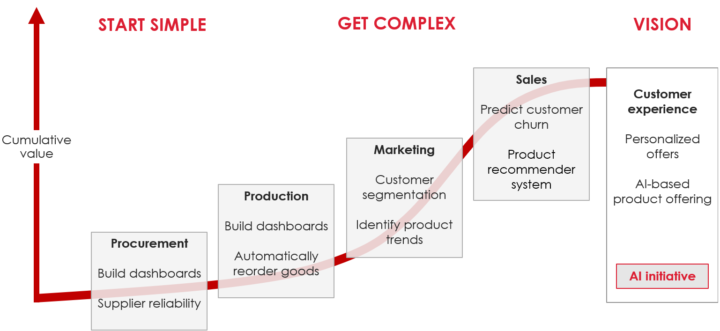
While many companies and businesses are investing in AI and machine learning to stay competitive and capture the untapped business opportunity, they are not reaping the benefits of those investments as their journey of operationalizing machine learning is stuck as a jupyter notebook level data science project. And that’s where MLOps comes to the rescue.
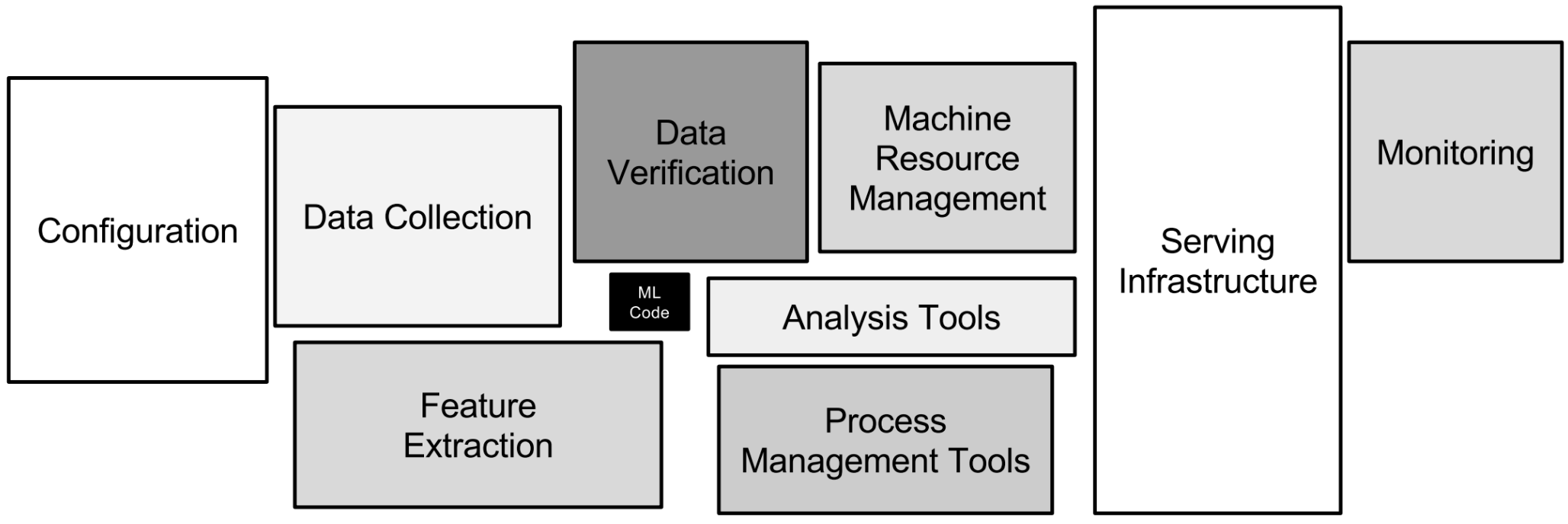
MLOps is a set of tools and practices for the development of machine learning systems. It aims to enhance the reliability, efficiency, and speed of productionizing machine learning. In the meantime, adhering to governance requirements. MLOps facilitate collaboration among data scientists, ML engineers, and other stakeholders and automate processes for a quicker production cycle of machine learning models. MLOps takes a few pages out of DevOps book; a methodology of modern software development but differs in asset management, as it involves managing source code, data, and machine learning models together for version control and model comparison, as well as for model reproducibility. Therefore, in essence, MLOps involves jointly managing source code (DevOps), data (DataOps) and Machine Learning models (ModelOps), while also continuously monitoring both the software system and the machine learning models to detect performance degradation.
MLOps = DevOps + DataOps + ModelOps
MLOps on Databricks
Recently, I had a chance to test and try out the Databricks platform. And in this blog post, I will attempt to summarise what Databricks has to offer in terms of MLOps capability.
First of all, what is Databricks ?
Databricks is a web based multi-cloud platform that aims to unify data engineering, machine learning, and analytics solutions under single service. The standalone aspect of Databricks is its LakeHouse architecture that provides data warehousing capabilities to a data lake. As a result, Databricks lakehouse eliminates the data silos due to pushing data into multiple data warehouses or data lakes, thereby providing data teams the single source of data.
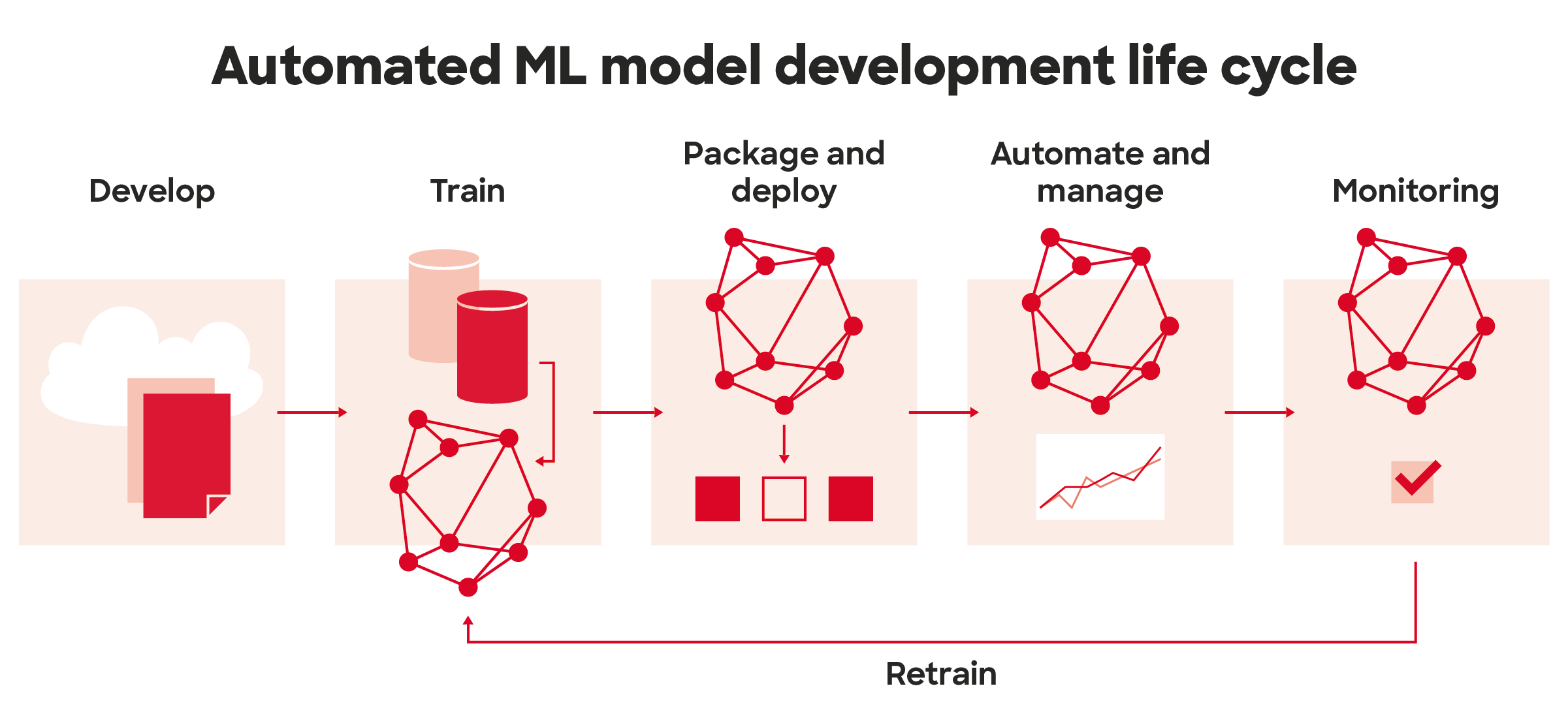
Databricks aims to consolidate, streamline and standardise the productionizing machine learning with Databricks Machine Learning service. With MLOps approach built on their Lakehouse architecture, Databricks provides suits of tools to manage the entire ML lifecycle, from data preparation to model deployment.
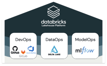
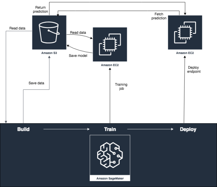
MLOps approach on Databricks is built on their Lakehouse Platform which involves jointly managing code, data, and models. Fig:Databricks
For the DevOps part of MLOps, Databricks provides capability to integrate various git providers, DataOps uses DeltaLake and for ModelOps they come integrated with MLflow: an open-source machine learning model life cycle management platform.
DevOps
Databricks provides Repos that support git integration from various git providers like Github, Bitbucket, Azure DevOps, AWS CodeCommit and Gitlab and their associated CI/CD tools. Databricks repos also support various git operations such as cloning a repository, committing. and pushing, pulling, branch management, and visual comparison of diffs when committing, helping to sync notebooks and source code with Databricks workspaces.
DataOps
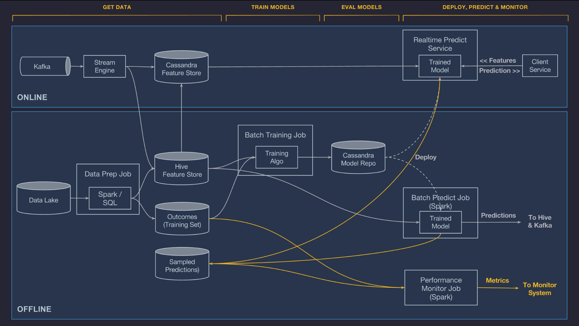
DataOps is built on top of Delta Lake. Databricks manages all types of data (raw data, log, features, prediction, monitoring data etc) related to the ML system with Delta Lake. As the feature table can be written as a Delta table on top of delta lake, every data we write to delta lake is automatically versioned. And as Delta Lake is equipped with time travel capability, we can access any historical version of the data with a version number or a timestamp.
In addition, Databricks also provides this nice feature called Feature Store. Feature Store is a centralised repository for storing, sharing, and discovering features across the team. There are a number of benefits of adding feature stores in machine learning learning development cycle. First, having a centralised feature store brings the consistency in terms of feature input between model training and inference eliminating online/offline skew there by increasing the model accuracy in production. It also eliminates the separate feature engineering pipeline for training and inference reducing the technical dept of the team. As the feature store integrates with other services in Databricks, features are reusable and discoverable to other teams as well; like analytics and BI teams can use the same set of features without needing to recreate them. Databricks’s Feature store also allows for versioning and lineage tracking of features like who created features, what services/models are using them etc thereby making it easier to apply any governance like access control list over them.
ModelOps
ModelOps capability in Databricks is built on a popular open-source framework called MLFlow. MLflow provides various components and apis to track and log machine learning experiments and manage model’s lifecycle stage transition.
Two of the main components of MLFlow are MLFlow tracking and MLFlow model registry.
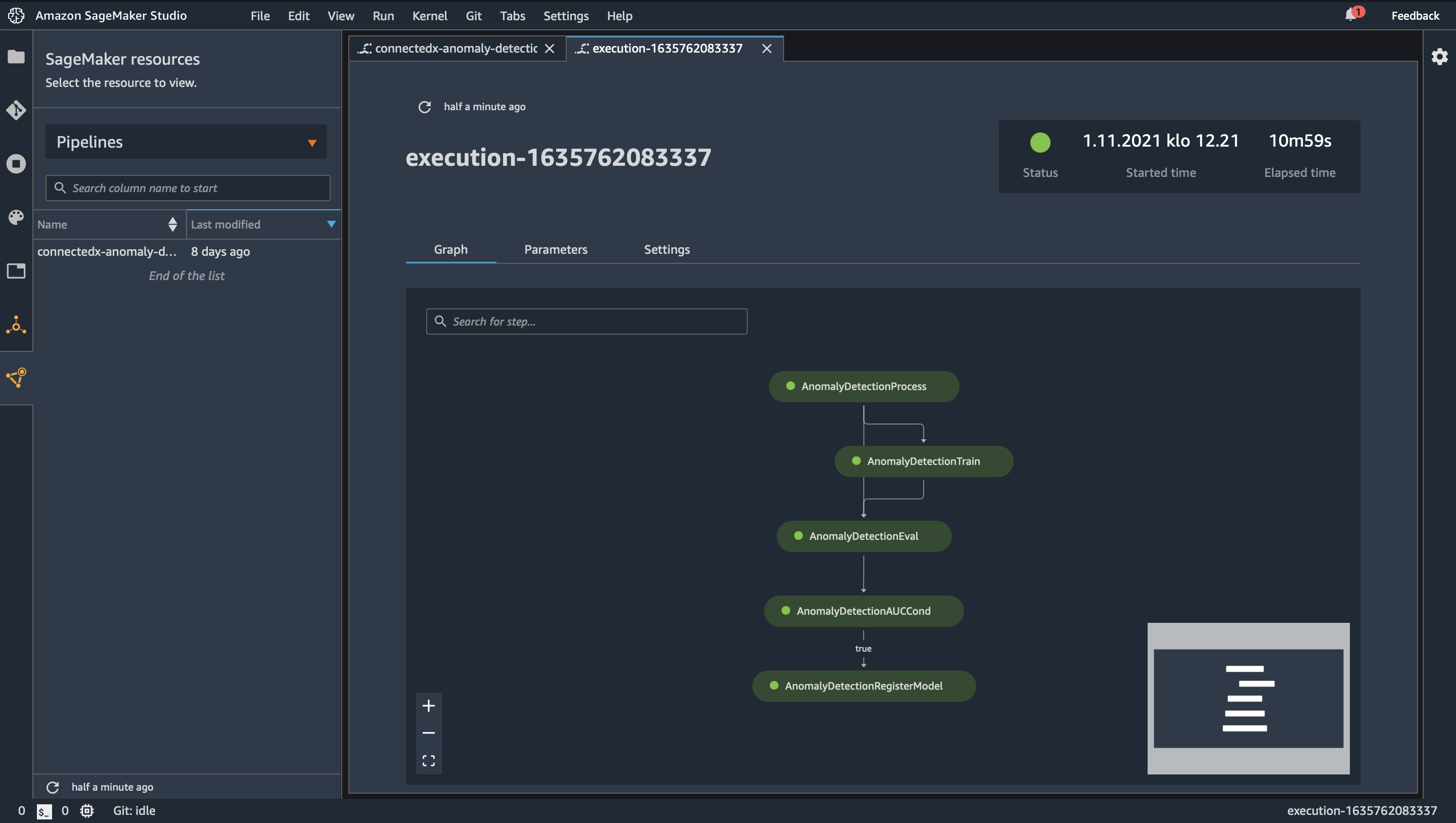
The MLflow tracking component provides an api to log and query and an intuitive UI to view parameters, metrics, tags, source code version and artefacts related to machine learning experiments where experiment is aggregation of runs and runs are executions of code. This capability to track and query experiments helps in understanding how different models perform and how their performance depends on the input data, hyperparameter etc.
Another core component of MLflow is Model Registry: a collaborative model hub, which let’s manage MLflow models and their lifecycle centrally. Model registry is designed to take a model from model tracking to put it through staging and into production. Model registry manages model versioning, model staging (assign “Staging” and “Production” to represent the lifecycle of a model version), model lineage (which MLflow Experiment and Run produced the model) and model annotation (e.g. tags and comments). Model registry provides webhooks and api to integrate with continuous delivery systems.
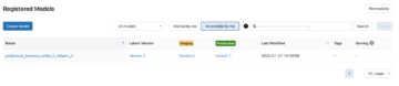
The MLflow Model Registry enables versioning of a single corresponding registered model where we can seamlessly perform stage transitions of those versioned models.
Databricks also supports the deployment of Model Registry’s production model in multiple modes: batch and streaming jobs or as a low latency REST API, making it easy to meet the specific requirements of an organisation.
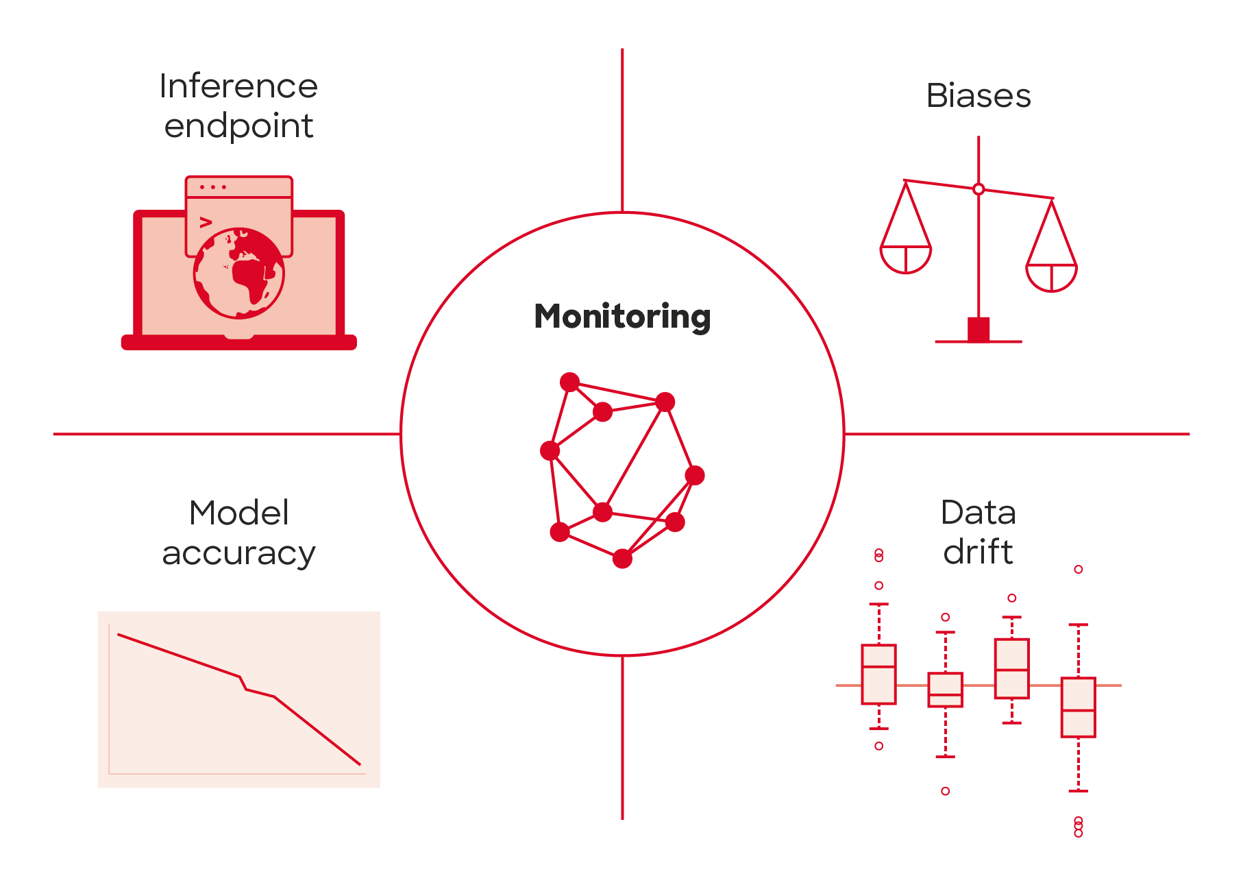
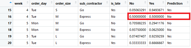
For model monitoring, Databricks allows logging the input queries and predictions of any deployed model to Delta tables.
Conclusion
MLOps is a relatively nascent field and there are a myriad of tools and MLOps platforms out there to choose from. Apples to apples comparison of those platforms might be difficult as the best MLOps tool for one case might differ to another case. After all, choosing the fitting MLOps tools highly depends on various factors like business need, current setup, available resources at disposal etc.
However, with the experience of using a few other platforms, personally, I find Databricks the most comprehensive platform of all. I believe Databricks make it easy for organisations to streamline their ML operations at scale. Platform’s collaboration and sharing capabilities should make it easy for teams to work together on data projects using multiple technologies in parallel. One particular tool which I found pleasing to work with is Databricks notebook. It is a code development tool, which supports multiple programming languages (R, SQL, Python, Scala ) in a single notebook, while also supporting real time co-editing and commenting. In addition, as the entire project can be version controlled by a tool of choice and integrates very well with their associated CI/CD tools, it adds flexibility to manage, automate and execute the different pipelines.
To sum up, Databricks strength lies in its collaborative, comprehensive and integrated environment for running any kind of data loads whether it is data engineering, data science or machine learning on top of their Lakehouse architecture. While many cloud based tools come tightly coupled with their cloud services, Databricks is cloud agnostic making it easy to set up if one’s enterprise is already running on a major cloud provider (AWS, Azure or Google cloud).
Finally, if you would like to hear more about Databricks as an unified Analytics, Data, and Machine Learning platform and learn how to leverage Databricks services in your Data journey, please don’t hesitate to contact me our Business Lead – Data Science, AI & Analytics, Mikael Ruohonen at +358414516808 or mikael.ruohonen@solita.fi or me at jyotiprasad.bartaula@solita.fi.