Do machines speak? Audio fingerprinting of internal combustion engines

Sensor data analytics is a fast-growing trend in the industrial domain. Audio, despite its holistic nature and huge importance to human machine operators, is usually not utilised to its full potential. In this blog post we showcase some of these possibilities through a research experiment case study conducted as part of the IVVES research project.

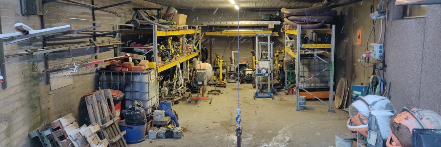
On a cold winter morning in December 2021 in the Solita Research R&D group we packed our bags with various audio recording equipment and set our sights on a local industrial machine rental company. We wanted to answer a simple question: do machines speak? Our aim was to record sound from multiple identical industrial grade machines (which turned out to be 53 kg soil compactors) in order to investigate whether we could consistently distinguish them based on their sound alone. In other words, just as each human has a very unique voice, our hypothesis was that the same would be true for machines, that is, we wanted to construct an audio fingerprint. This could then be used not only to identify each machine, but to detect if a particular machine’s sound starts to drift (indicating a potential incoming fault) or to check whether the fingerprint matches before and after renting out the machine, for example.

It is always important to keep the business use case and real-world limitations in mind when designing solutions to data-based (no pun intended) problems. In this case, we identified the following important aspects in our research problem:

  1. The solution would have to be lightweight, capable of being run on the edge with limited computational resources and internet connectivity.
  2. Our methods should be robust against interference from varying levels of background noise and variances in how users hold the microphone when recording a machine’s sound.
  3. It would be important to be able to communicate our results and analysis to domain experts and eventual end users. Therefore, we should focus on physically meaningful features over arbitrary ones and on explainable algorithms over black boxes.
  4. The set-up of our experiment should be planned to ensure high-quality uncontaminated data that at the same time would serve to produce the best possible research outcome while being representative of the data we might expect for a productionalised solution.

In this blog post we will focus on points 1. and 3. and we’ll return to 2. and 4. in a follow-up post.

Analysing Sound

We are surrounded by a constant stream of sound mixed together from a multitude of sources: cars speeding along on the street, your colleague typing on their keyboard or a dog barking at songbirds outside your window. Yet, seemingly without any effort, your brains can process this jumbled up signal and tell you exactly what is happening around you in real-time. Our hope is that we could somehow imitate this process by developing audio analysis methods with similar properties.

Waveform of speech on the left, corresponding spectrogram on the right.
Figure 1. On the left is the waveform for the sound produced by the author uttering “hello”. On the right is the corresponding spectrogram.

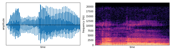
It is quite futile to try to analyse raw signals of this type directly: each sound source emits vibrations in multiple frequencies and these get combined over all the different sources into one big mess. Luckily there is a classical mathematical tool which can help us to figure out the frequency content of an audio (or any other type) wave: the Fourier transform. By computing the Fourier transform for consecutive small windows of the input signal, we can determine how much of each frequency is present at a given time. We can then arrange this data in the form of a matrix, where the rows correspond to different frequency ranges and columns are consecutive time steps (typically in the order of 10-20 milliseconds each). Hence, the entries of the matrix tell you how much of each frequency is present at that particular moment. The resulting matrix is called a spectrogram, which we can visualise by colouring the values based on their magnitudes: dark for values close to zero with lighter colours signifying higher intensity. In Figure 1 you can see an example of the waveform produced by the author uttering “hello” and the resulting spectrogram. The process of transforming the original signal to its constituent frequencies and studying this decomposition is called spectral analysis.

From Raw to Refined Features

The raw frequency data by itself is still not the most useful. This is because different audio sources can of course produce sounds in overlapping frequency ranges. In particular, a single machine can have multiple vibrating parts which each produce their distinct sound. Instead, we should try to extract features that are meaningful to the problem at hand—classification of fuel powered machines in this case. There are many spectral features that could be useful (for some inspiration you can check out our public Google Colab notebooks or the documentation of librosa, a popular Python audio analysis library).

In this blog we’ll take a slightly different approach. Our goal is to be able to compare the frequency data of different machines at two points in time, but this won’t be efficient (let alone robust) if we rely on raw frequencies. This is because of background noise and the varying operating speed of the engines (think about how the pitch of the sound is affected by how fast the engine is running). Instead, we want to pool together individual frequencies in a way that would allow us to express our high-dimensional spectrogram in terms of a handful of distinct frequency range combinations.

Weights of the coefficients for the first two principal components.
Figure 2. Each principal component is some combination of frequencies with different weights.

Luckily there is, yet again, a classical mathematical tool which does exactly this: principal component analysis (PCA). If you’ve taken a course in linear algebra then this is nothing more than matrix diagonalisation, but it has become one of the staple methods of dimensionality reduction in the machine learning world. The output of the PCA-algorithm is a set of principal components each of which is some combination of the original frequencies. In Figure 2 we plot the weight of each frequency for two principal components: in the first component we have positive weights for all but the lowest of frequencies while for the second one the midrange has negative weights. An additional reason for why PCA is an attractive method for our problem is that the resulting frequency combinations will be linearly independent (i.e. you cannot obtain one component by adding together multiples of the other components). This is a crude imitation of our earlier observation that a single machine can have multiple separate parts producing sound at the same time. The crux of the algorithm is that in order to faithfully represent our original data, we only have to keep a small number of these principal components thus effectively reducing the dimensionality of our problem to a more manageable scale.

Structure in Audio

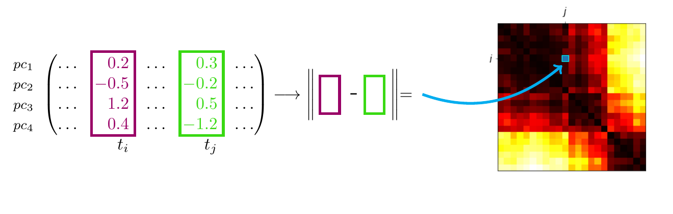
Now that we have a sequence of low-dimensional feature vectors that capture the most important aspects of the original signal, we can try to start finding some structure in this stream of data. We do this by computing the self-similarity matrix (SSM) [1], whose elements are the pairwise distances between our feature vectors. We can visualise the resulting matrix as a heat map where the intensity of the colour corresponds to the distance (with black colour signifying that the features are identical), see Figure 3.

Showing how the self-similarity matrix is obtained from the feature vectors via pairwise distances.
Figure 3. The (i, j)-entry of the self-similarity matrix (on the right) is given by the distance between the feature vectors at times ti and tj. Black colour corresponds to zero distance i.e. the vectors being equal.

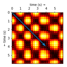
In Figure 4 you can see a part of an SSM for one of the soil compactors. By definition, time flows along its main diagonal (blue arrow). Short segments of the audio that are self-similar (i.e. the nature of the sound doesn’t change) appear as dark rectangles along the diagonal. For each rectangle on the main diagonal, the remaining rectangles on the same row show how similar the other segments are to the one in question. If you pause here for a moment and gather your thoughts, you might notice that there are two types of alternating segments (of varying duration) in this particular SSM.

Self-similarity matrix for a soil compactor showcasing an repeating pattern of two alternating segments.
Figure 4. Self-similarity matrix for one of the soil compactors. Time flows down the main diagonal on which the dark rectangles signify self-similar segments.

Do machines speak?

We have covered a lot of technical material, but we are almost done! Now we understand how to uncover patterns in audio, but how can we use this information to tell apart our four machines? The more ML-savvy readers might be tempted to classify the SSMs with e.g. convolutional neural networks. This might certainly work well, but we would lose sight of one of our aims which was to keep the method computationally light and simple. Hence we proceed with a more traditional approach.

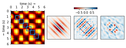
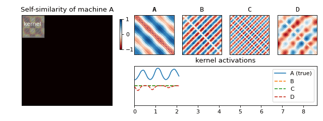
Recall that we have constructed a separate SSM for each machine. For each of the resulting matrices, we can now look at small blocks along the diagonal (see Figure 5) and figure out what they typically look like. If we scale the results to [-1, 1], we obtain a small set of fingerprints (we also refer to these as kernels) for each machine. Just like you (hopefully) have ten fingers each with its own unique fingerprint, a machine can also have more than one acoustic fingerprint. We have visualised a few of these for one of the machines in Figure 5.

Fingerprints (on the right) for a single machine computed from its self-similarity matrix on the left.
Figure 5. Fingerprints (on the right) for a single machine computed from its self-similarity matrix on the left.

We are now ready to return back to the machine rental shop to test if our solution works! Once we arrive, we follow the set of instructions below in order to determine which machine is which (see Figure 6 for an animation of this process):

  1. Turn on the machine and record its sound.
  2. While the machine is running, compute the self-similarity matrix on the fly.
  3. Slide the fingerprints for each machine along the diagonal and compute their activations (by summing the elementwise product).
  4. The fingerprint which reacts to the sound the most tells you which machine is running.
By computing the activations of each fingerprint on freshly recorded audio, we can find out which machine has been returned to the rental shop.
Figure 6. By computing the activations of each fingerprint on freshly recorded audio, we can find out which machine has been returned to the rental shop.

And that’s it! We saw how something seemingly natural, the sounds surrounding us, can produce very complex signals. We learned how to begin to understand this mess via spectral analysis, which led us to uncover structure hidden in the data—something our brain does with ease. Finally, we used this structure to produce a solution to our original business use case of classifying machine sounds.

I hope you have enjoyed this little excursion into the mathematical world of audio data and colourful graphs. Maybe next time you start your car (or your soil compactor) you might wonder whether you could recognise its sound from your neighbour’s identical one and what it is about their sounds that lets your brain achieve that.

If you are interested in applying advanced sensor data (audio or otherwise) analytics in your business context please reach out to me or the Solita Industrial team.

References

[1] J. Foote, Visualizing Music and Audio using Self-Similarity, MULTIMEDIA ’99, pp. 77-80 (1999) http://www.musanim.com/wavalign/foote.pdf


Solita Health researched: Omaolo online symptom checker helps to predict national healthcare admissions related to COVID-19

In our recently published study [1], I and my Solitan colleagues Kari Antila and Vilma Jägerroos examined the possibility of predicting the burden of healthcare using machine learning methods. We used data on symptoms and past healthcare utilization collected in Finland. Our results show that COVID-19-related healthcare admissions can be predicted one week ahead with an average accuracy of 76% during the first wave of the pandemic. Similar symptom checkers could be used in other societies and for future epidemics, and they could provide an opportunity to collect data on symptom development very rapidly - and at a relatively low cost.

The rapid spread of the SARS-CoV-2 virus in March 2020 presented challenges for nationwide assessment of the progression of the COVID-19 pandemic. In Finland, Solita helped to add a COVID-19 symptom checker to a pre-existing national, CE-marked medical symptom checker service ©Omaolo. The Omaolo COVID-19 symptom checker achieved considerable popularity immediately after its release, and the city of Helsinki, for example, has estimated annual savings of 2.5 million euros from its use. Although there have been studies about how well symptom checkers perform as clinical tools, their data’s potential on predicting epidemic progression, to our knowledge, has not yet been studied.

For this purpose, Solita developed a machine learning pipeline in the Finnish Institute for Health and Welfare’s (THL) computing environment for automated model training and comparison. The models created by Solita were retrained every week using time-series nested cross-validation, allowing them to adapt to the changes in the correlation of the symptom checker answers and the healthcare burden. The pipeline makes it easy to try new models and compare the results to previous experiments. 

We decided to compare linear regression, a simple and traditional method, to XGBoost regression, a modern option with many hyperparameters that can be learned from the data. The best linear regression model and the best XGBoost model (shown in the figure) achieved mean absolute percentage error of 24% and 32%, respectively. Both models get more accurate over time, as they have more data to learn from when the pandemic progresses.

COVID-19–related admissions predicted by linear regression and XGBoost regression models, together with the true admission count during the first wave of the pandemic in 2020.

Our results show that a symptom checker is a useful tool for making short-term predictions on the health care burden due to the COVID-19 pandemic. Symptom checkers provide a cost-effective way to monitor the spread of a future epidemic nationwide and the data can be used for planning the personnel resource allocation in the coming weeks. The data collected with symptom checkers can be used to explore and verify the most significant factors (age groups of the users, severity of the symptoms) predicting the progression of the pandemic as well.

You can find more details in the publication [1]. The research was done in collaboration with University of Helsinki, Finnish Institute for Health and Welfare, Digifinland Oy, and IT Centre for Science, and we thank everyone involved.

If you have similar register data and would like to perform a similar analysis, get in touch with me or Solita Health and we can work on it together!

Joel Röntynen, Data Scientist, joel.rontynen@solita.fi

References

[1] ​​Limingoja L, Antila K, Jormanainen V, Röntynen J, Jägerroos V, Soininen L, Nordlund H, Vepsäläinen K, Kaikkonen R, Lallukka T. Impact of a Conformité Européenne (CE) Certification–Marked Medical Software Sensor on COVID-19 Pandemic Progression Prediction: Register-Based Study Using Machine Learning Methods. JMIR Form Res 2022;6(3):e35181, doi: 10.2196/35181, PMID: 35179497

Reading the genomic language of DNA using neural networks

Neural networks are powerful tools in natural language processing (NLP). In addition, they can also learn the language of DNA and help in genome annotation. Annotated genes, in turn, play a key role in finding the causes and developing treatments for many diseases.

I have been finishing my studies while working at Solita and got the opportunity to do my master’s thesis in the ivves.eu research program in which Solita is participating. The topic of my thesis consisted of language, genomics and neural networks, and this is a story of how they all fit into the same picture.

When I studied Data Science at the University of Helsinki, courses in NLP were my favorites. In NLP, algorithms are taught to read, generate, and understand language, in both written and spoken forms. The task is difficult because of the characteristics of the language: words and sentences can have many interpretations depending on the context. Therefore, the language is far from accurate calculations and rules where the algorithms are good at. Of course, such challenges only make NLP more attractive!

Neural networks

This is where neural networks and deep learning come into play. When a computational network is allowed to process a large amount of text over and over again, the properties of the language will gradually settle into place, forming a language model. A good model seems to “understand” the nuances of language, although the definition of understanding can be argued, well, another time. Anyways, these language models taught with neural networks can be used for a wide variety of NLP problems. One example would be classifying movie reviews as positive or negative based on the content of the text. We will see later how the movie reviews can be used as a metaphor for genes.

In recent years, a neural network architecture called transformers has been widely used in NLP. It utilizes a method called attention, which is said to pay attention to emphases and connections of the text (see the figure below). This plays a key role in building the linguistic “understanding” for the model. Examples of famous transformers (other than Bumblebee et al.) include Google’s BERT and OpenAI’s GPT-3. Both are language models, but transformers are, well, transformable and can also be used with inputs other than natural language.

An example of how transformers self-attention “sees” the connections in a sentence. The difference of the last word completely changes what the word “it” most refers to.


DNA-language

And here DNA and genomes come into the picture (also literally in the picture below). You see, DNA has its own grammar, semantics, and other linguistic properties. At its simplest, genes can be thought of as positive movie reviews, and non-coding sequences between genes as negative reviews. However, because the genomes of organisms are part of nature, genes are a little more complex in reality. But this is just one more thing that language and genomics have in common: the rules do not always apply and there is room for interpretation.

Simplification of a genome and a gene. Genomic data is a long sequence of characters A, T, C, and G representing four nucleotide types. Genes are coding parts of the genome. At their simplest, they consist of start and end points and the characters between them.


Since both text and genomic data consist of letters, it is relatively straightforward to teach the transformer model with DNA sequences instead of text. Like the classification of movie reviews in an NLP-model, the DNA-model can be taught to identify different parts of the genome, such as genes. In this way, the model gains the understanding of the language of DNA.

In my thesis, I used DNABERT, a transformer model that has been pre-trained with a great amount of genomic data. I did my experiments with one of the most widely known genomes, E. coli bacterium, and fine-tuned the model to predict its gene locations.

Example of my experiments: the Receiver operating characteristic (ROC) curves helped me to find the most optimal input length for the genome data. Around 100 characters led to the highest curve and thus the best results, whilst 10 was obviously too short and 500 too long.

After finding the most optimal settings and network parameters, the results clearly showed the potential. Accuracy of 90.15% shows that the model makes “wise” decisions instead of just guessing the locations of the genes. Therefore the method has potential to assist in the basic task of bioinformatics: new genomes are sequenced at a rapid pace, but their annotation is slower and more laborious. Annotated genes are used, for example, to study the causes of diseases and to develop treatments tailored to them.

There are also other methods for finding genes and other markers in DNA sequences, but neural networks have some advantages over more traditional statistics and rule based systems. Rather than human expertise in genomics, the neural network based method relies on the knowledge gathered by the network itself, using a large amount of genomic data. This saves time and expert hours in the implementation of the neural network. The use of the pre-trained general DNA language model is also environmentally friendly. Such a model can be fine-tuned with the task-specific data and settings in just a few iterations, saving computational resources and energy. 

There is a lot of potential in further developing the link between transformer networks and DNA to study what else the genome language has to tell us about the life around us. Could this technology contribute to the understanding of genetic traits, the study of evolution, the development of medicine or vaccines? These questions are closely related to the healthcare field, in which Solita has strong expertise, including in research. If you are interested in this type of research, I and other Solita experts will be happy to tell you more!

Venla Viljamaa (Data Scientist) venla.viljamaa@solita.fi linkedin.com/in/venlav/