AWS forecast service modelling Electricity consumption

Timeseries forecasting often requires significant mathematical knowledge and domain experience. This area of machine learning is often only accessible to experts, however, Amazon Forecast provides a simple and intuitive interface for creating complex machine learning models.

Timeseries forecasting is the process of looking at historical data to make predictions about the future. Companies can use these predictions to extract actionable insights that drive innovation. Often, the mechanisms behind the transformation of raw data into business value is a mystery to non-specialists. This is because timeseries forecasting requires expert knowledge of algorithms and mathematical concepts such as calculus. This is a domain reserved for the highly trained specialists, often not accessible to the average user. However, with the development of Amazon Forecast this could be changing.

Amazon Forecast is a fully managed service that simplifies the process of timeseries forecasting by hiding the inner complexity from the users. The user simply has to provide an input data, Forecast then automatically applies and selects the most optimal machine learning algorithm for the data to generate accurate predictions with little to no user intervention. This system is known as a ‘Black Box Method’, where a user can conduct complex modelling tasks without worrying about the low-level calculus and algorithms.

This movement of machine learning from experts to general users marks a significant paradigm shift known as AutoML (Automatic Machine Learning).

Within this blog Amazon Forecast will be explored from the perspective of a non-expert general user to assess how easy it is to get started producing accurate future predictions. In other words, can someone who is not a professional machine learning specialist produce professional models?

What we will predict

In this hypothetical scenario we work for an electricity provider and have been tasked with building a model to predict future electricity consumption for our customers. The input data we have been provided contains measurements for electricity consumption (Kw) every hour for 370 different clients from January 2014 – November 2014. This dataset contains 2,707,661 observations. We will build a model to predict the electricity consumption for the 1st of October 2014, so 24 hours into the future for every customer.

Creating the electricity forecast

 Unfortunately, Forecast is not able to clean and prepare your input data, you must ensure the data is prepared beforehand. This is the only technical step that is required in the forecasting process. In this instance, we prepare the dataset to match the schema requirements of Forecast as shown in the table below. Once prepared the data must be stored in an S3 as a CSV.


Client Timestamp Consumption
Client_1 2014-01-01 01:00:00 23.64
Client_0 2014-0101 02:00:00 9.64


As a general user we can achieve everything we need to generate a forecast within the Forecast Console. This is a no-code user interface in the form of a Dashboard. Within this dashboard we can manage all aspects of the forecasting process, this process is implemented in 3 easy steps:

  1.   First, you import your Target time series data. This is simply the process of telling Forecast where to find your prepared data in S3 and how to read the contents (schema).
  2.       Next, you use this Target time series to create a predictor. A predictor is a Forecast model trained on your timeseries. This is where the AutoML aspects of Forecast are truly utilised. When training a predictor in a typical timeseries forecast, the user would need to identify the optimal algorithm to train the model and then optimise this model. Within Forecast, all of these steps are done automatically using back testing. Back testing is the process of retaining a portion of the training data to train on all the algorithms to find the best fit.
  3.       Finally, with the model trained, we can generate a forecast. This is as simple as a few clicks on the dashboard. This will generate future predictions of energy consumption for every hour for every customer.

Now, with zero coding or expert input we have generated an advanced forecast utilising cutting-edge deep learning machine learning algorithm. If it appears very simple, that’s because it is. The dashboard was designed to be simple and easy to use. For more advanced users Python can be used to connect to Forecast where you gain significantly more control over the process. But as a general user such control is not necessary.

Visualise and export the electricity consumption predictions

For this section we will visualise the forecasted predictions for customer 339, found in the graph below. As we actually have the real observed values for the 1st of October 2014, we can compare our predictions with the actual observed electricity consumption.

In the graph the darker blue line represents the real values. We can also see a red line and a light blue area. This blue area is known as the 80% confidence interval, indicating that we are 80% confident that the real value will lie somewhere within this area. The red line, p50 value (median forecast) can be considered as an indication of the ‘most likely outcome’.

As we can see, our forecast appears to be very accurate in predicting the electricity consumption for this customer, with the predicted values closely following the observed values. In practice, these forecasts could be used in a variety of ways. For example, we could share this forecast with the customer, who can then adjust their consumption patterns to reduce energy usage during peak hours and thus lower energy bills. For the energy provider, these forecasts could be used in load management and capacity planning.

Conclusion

The main purpose of Forecast and AutoML is to allow non-experts to develop machine learning models without the required expertise. AutoML also enables experienced data scientists by reducing time spent optimising models. Forecast achieves both, as I, a non-expert, was able to develop an advanced forecasting model without any interaction with the complex underlying mechanisms. It is clear Forecast extends the power of time series forecasting to non-technical experts, empowering them to make informed decisions from machine learning insights.

AI Act is coming. Is your organisation ready?

EU regulation called AI Act is fast approaching and will regulate how artificial intelligence is used in the EU. This blog post looks at what each organisation should be doing to be prepared in time for this.

The EU regulation on ethical and robust AI solutions called the AI Act is fast approaching. The idea behind this regulation is to enable the development of artificial intelligence while ensuring that human rights are considered and accounted for in the development. The current estimated timeline is to reach an agreement about the content of the AI Act with all member states by the end of this year and have it in effect soon after. The broad strokes of this regulation are already known. My advice for all organisations is to start preparing for this now. 

Two ways to prepare for the AI Act 

The first thing is to become educated on what this regulation is and make sure everyone in your organisation creating, developing, and deciding on AI projects is also aware of it. This relates to the reasons behind it, the broad strokes of the regulation itself, and how to prepare for it. 

The second aspect focuses on preparing the AI solutions in the development pipeline and in production to comply with the regulation as well as also looking at the development culture in the organisation so new AI solutions can be compliant by design. We at Solita have developed a client-tested tool and framework to help with this.

I will also look more closely at both topics next.

Get educated: how we got here and where’s here?

News of companies running into ethical and legal problems with artificial intelligence has made headlines for years with increasing numbers. In 2016 The COMPAS risk assessment recidivism algorithm used by the U.S. court system was assessed to be very biased. Microsoft unveiled the Tay chatbot only to take it offline within 16 hours due to inflammatory and offensive tweets. In 2018 Amazon shut down their recruitment AI for sexist results and in 2019 Apple credit card ran into problems when it offered smaller lines of credit to women than to men.

These and similar issues as well as the rise in popularity of this technology quickly put this topic on the tables of regulators to regulate AI in a way to make it align with legal, ethical, and safety guidelines in the European Union.

The rise in popularity of generative AI, with f.ex. Midjourney and ChatGPT, has required discussions on the content and wording of the AI Act late in this process.

In June 2018 the European Commission established an expert group to create Ethics Guidelines for Trustworthy Artificial Intelligence. The group emphasized three key components for the development of AI. Firstly, AI solutions should be lawful, adhering to existing laws and regulations related to, for instance, product development, data usage, and discrimination. Secondly, AI should be ethical, respecting principles of human autonomy, prevention of harm, fairness, and explicability. Lastly, AI systems should be technically robust, safe, and secure, and consider their social environment. Particular attention should be given to vulnerable and historically disadvantaged groups and situations characterized by power or information imbalances.

In April 2021 the European Commission proposed the first EU regulatory framework for AI. Their priority was to make sure that AI systems used in the EU are safe, fair, transparent, traceable, non-discriminatory, overseen by people, and environmentally friendly. This proposed framework is the basis of the AI Act. Since June 2023, the regulation has transitioned to the phase where EU countries are forming the final wording of the regulation.

General principles of this regulation is that all AI systems are safe, protect privacy, transparent, and non-discriminate, as well as having proper data management.

The plan is to reach an agreement by the end of this year with Generative AI causing plenty of discussions this spring.

The regulation takes a use case-based approach categorizing AI applications into four risk levels, which are low, limited, high and unaccepted risk. Low-risk applications, such as email spam filters and predictive maintenance systems, are not heavily regulated but still encouraged to be robust. Limited risk applications, including chatbots, are subject to transparency obligations. Users must be aware that they are interacting with AI and should have the option to discontinue use while at the same time receiving the service. 

Generative AI can be at different risk levels. If used in low-risk application, it needs to be transparent in disclosing AI-generated content for users, prevent the generation of illegal content, and publish summaries of copyrighted data used in training. Currently, the larger foundational models still somewhat lack these aspects as Stanford University discovered earlier this year. The companies providing general-purpose foundational models AIs like GPT have requirements stated if they are to operate within EU. 

High-risk applications are such that the system poses a significant risk of harm to the health, safety, or fundamental rights of natural persons or the environment and are subjected to strict obligations throughout their lifecycle. These use cases are defined as AI systems in law enforcement, migration and border control, recommender systems of large online platforms, justice administration and democratic processes, education, employment, essential private and public services, and critical infrastructure. These systems require comprehensive risk assessments and mitigation, data governance practices, transparency and provision of information about it being an AI system. They also require a fundamental rights impact assessment and monitoring environmental impact. 

The unaccepted risk and hence prohibited use cases pose clear threats to people’s safety, livelihoods, and rights. Examples include biometric classification of individuals based on sensitive characteristics, real-time remote biometric identification and retrospective identification from recordings, proactive policing activities, emotion recognition systems in f.ex. law enforcement and education, and establishing large-scale facial recognition databases. These will not be allowed within the EU. 

Get prepared: finding and fixing potential issues 

While education on the regulation is still happening, the review of AI use cases in development and production should take place. This involves all solutions that are being designed, are in development, or are in production. For each, an assessment should be done on their risk level according to the regulation and the priority for business of each solution. This is a fairly simple operation of having current the AI Act guidelines and looking through each use case to which category they are most likely to land in. Legal advice can be sought to offer guidance in cases that could be seen one way or the other. For solutions in production that are already GDPR compliant and not high-risk, the chances are that required chances are small.

After each solution has been classified to a risk level, the characteristics of each solution need to be investigated regarding the AI Act risk assessment classification. We have developed a customer-tested framework and tool for this at Solita. The list of things to look at is very different in a low-risk application to that of a high-risk application. I recommend starting with the business-critical applications first. The idea here is to foresee possible issues with complying with the regulation and react to them in descending order of priority. 

One thing each organisation should consider. If you are using an AI system offered from outside the EU, but used inside the EU, it’s advisable to prepare for some interruption of service.  Systems offered outside the EU might not all choose to comply with the regulation but will instead opt out and not offer their services inside the EU, or they might take their service offline while building compliance with the new regulation. The more critical the AI system is to the company, the more important it is to take this into account in time.

Review the development and maintenance pipeline

While reviewing each use case is important, it is important also to start building or strengthening processes that ensure compliance with the regulation now and in the future so AI solutions can be compliant by design. Our framework serves this process well. The tool allows a company to look at their AI development processes, as well as each model, to easily document the current ways of working, identify any issues needing further development, and a way to document progress against identified gaps. We are closely following the development of the regulation and developing the framework accordingly.

Build a roadmap and implement it

Once use cases have been identified and the ways of working assessed, the next phase is to develop a roadmap in order of priority to fix any identified issues before they cause problems. Our framework helps with this. In limited to no-risk use cases it is useful to already start building transparency of an AI model being used and start building opt-out methods if not already present. Also, and especially in high-risk use cases, building a method of redress and obtaining explanations of the decisions made by the AI system, is very important.

For any use case that can be considered high risk, a more thorough investigation should be already started that documents carefully the system and its development and provides users and affected parties with the necessary information on the solution. The Solita framework makes this process easier. For the forbidden use cases, if they exist, it is necessary to think about the end of life of these solutions. 

Act now

The AI Act is coming, and it is coming soon. I recommend starting to prepare for it now, and, if necessary, seek out ML engineers, responsible AI experts, and designers with thorough knowledge and understanding of this topic area to help to educate staff and build a roadmap for compliance with each AI solution in the development pipeline or in production. When the regulation comes into effect, I suspect many organizations will wake up to the need to do something as they did when GDPR came into effect and consultancies capable of helping them will be fully booked quickly.  As the main parts of this regulation are already well known, my advice is to start preparing for this now. We’re always happy to help with client-tested tools to do so.

Oh, by the way, the Data Act, AI liability act, and Cyber Resiliency Act are coming too. Luckily, we’re looking at those too when we build our tools and frameworks.

MLOps on Databricks: Streamlining Machine Learning Workflows

Databricks is a cloud-based platform that seamlessly integrates data engineering, machine learning, and analytics to simplify the process of building, training, and deploying Machine Learning models. With its unified platform built on top of Lakehouse architecture, Databricks empowers Data Scientist and ML engineers to unleash their full potential, providing a collaborative workspace and offering comprehensive tooling that streamline the entire ML process, including tools to support DevOps to model development, deployment and management.

MLOps in a nutshell 

While many companies and businesses are investing in AI and machine learning to stay competitive and capture the untapped business opportunity, they are not reaping the benefits of those investments as their journey of operationalizing machine learning is stuck as a jupyter notebook level data science project. And that’s where MLOps comes to the rescue.

MLOps is a set of tools and practices for the development of machine learning systems. It aims to enhance the reliability, efficiency, and speed of productionizing machine learning. In the meantime, adhering to  governance requirements. MLOps facilitate collaboration among data scientists, ML engineers, and other stakeholders and automate processes for a quicker production cycle of machine learning models. MLOps takes a few pages out of DevOps book; a methodology of modern software development but differs in asset management, as it involves managing source code, data, and machine learning models together for version control and model comparison, as well as for model reproducibility. Therefore, in essence, MLOps involves jointly managing source code (DevOps), data (DataOps) and Machine Learning models (ModelOps), while also continuously monitoring both the software system and the machine learning models to detect performance degradation.


                                   MLOps = DevOps + DataOps + ModelOps


MLOps on Databricks

Recently, I had a chance to test and try out the Databricks platform. And in this blog post, I will attempt to summarise what Databricks has to offer in terms of MLOps capability. 

First of all, what is Databricks ? 

Databricks is a web based multi-cloud platform that aims to unify data engineering, machine learning, and analytics solutions under single service. The standalone aspect of Databricks is its LakeHouse architecture that provides data warehousing capabilities to a data lake. As a result, Databricks lakehouse eliminates the data silos due to pushing data into multiple data warehouses or data lakes, thereby providing data teams the single source of data. 

Databricks aims to consolidate, streamline and standardise the productionizing machine learning with Databricks Machine Learning service. With MLOps approach built on their Lakehouse architecture, Databricks provides suits of tools to manage the entire ML lifecycle, from data preparation to model deployment.

MLOps approach on Databricks is built on their Lakehouse Platform which involves jointly managing code, data, and models. Fig:Databricks

MLOps approach on Databricks is built on their Lakehouse Platform which involves jointly managing code, data, and models. Fig:Databricks

For the DevOps part of MLOps, Databricks provides capability to integrate various git providers, DataOps uses DeltaLake and for ModelOps they come integrated with MLflow: an open-source machine learning model life cycle management platform. 


DevOps 

Databricks provides Repos that support git integration from various git providers like Github, Bitbucket, Azure DevOps, AWS CodeCommit and Gitlab and their associated CI/CD tools. Databricks repos also support various git operations such as cloning a repository, committing. and pushing, pulling, branch management, and visual comparison of diffs when committing, helping to sync notebooks and source code with Databricks workspaces.


DataOps

DataOps is built on top of Delta Lake. Databricks manages all types of data (raw data, log, features, prediction, monitoring data etc) related to the ML system with Delta Lake. As the feature table can be written as a Delta table on top of delta lake, every data we write to delta lake is automatically versioned. And as Delta Lake is equipped with time travel capability, we can access any historical version of the data with a version number or a timestamp. 

In addition, Databricks also provides this nice feature called Feature Store. Feature Store is a centralised repository for storing, sharing, and discovering features across the team. There are a number of benefits of adding feature stores in machine learning learning development cycle. First, having a centralised feature store brings the consistency in terms of feature input between model training and inference eliminating online/offline skew there by increasing the model accuracy in production. It also eliminates the separate feature engineering pipeline for training and inference reducing the technical dept of the team. As the feature store integrates with other services in Databricks, features are reusable and discoverable to other teams as well; like analytics and BI teams can use the same set of features without needing to recreate them. Databricks’s Feature store also allows for versioning and lineage tracking of features like who created features, what services/models are using them etc thereby making it easier to apply any governance like access control list over them.


ModelOps

ModelOps capability in Databricks is built on a popular open-source framework called MLFlow. MLflow provides various components and apis to track and log machine learning experiments and manage model’s lifecycle stage transition. 

Two of the main components of MLFlow are MLFlow tracking and MLFlow model registry. 

The MLflow tracking component provides an api to log and query and an intuitive UI to view parameters, metrics, tags, source code version and artefacts related to machine learning experiments where experiment is aggregation of runs and runs are executions of code. This capability to track and query experiments helps in understanding how different models perform and how their performance depends on the input data, hyperparameter etc. 

Another core component of MLflow is Model Registry: a collaborative model hub, which let’s manage MLflow models and their lifecycle centrally. Model registry is designed to take a model from model tracking to put it through staging and into production. Model registry manages model versioning, model staging (assign “Staging” and “Production” to represent the lifecycle of a model version), model lineage (which MLflow Experiment and Run produced the model) and model annotation (e.g. tags and comments). Model registry provides webhooks and api to integrate with continuous delivery systems.

The MLflow Model Registry enables versioning of a single corresponding registered model where we can seamlessly perform stage transitions of those versioned models.


The MLflow Model Registry enables versioning of a single corresponding registered model where we can seamlessly perform stage transitions of those versioned models.

Databricks also supports the deployment of Model Registry’s production model in multiple modes: batch and streaming jobs or as a low latency REST API, making it easy to meet the specific requirements of an organisation.

For model monitoring, Databricks allows logging the input queries and predictions of any deployed model to Delta tables.

Conclusion

MLOps is a relatively nascent field and there are a myriad of tools and MLOps platforms out there to choose from. Apples to apples comparison of those platforms might be difficult as the best MLOps tool for one case might differ to another case. After all, choosing the fitting MLOps tools highly depends on various factors like  business need, current setup, available resources at disposal etc. 

However, with the experience of using a few other platforms, personally, I find Databricks the most comprehensive platform of all. I believe Databricks make it easy for organisations to streamline their ML operations at scale. Platform’s collaboration and sharing capabilities should make it easy for teams to work together on data projects using multiple technologies in parallel. One particular tool which I found pleasing to work with is Databricks notebook. It is a code development tool, which supports multiple programming languages (R, SQL, Python, Scala ) in a single notebook,  while also supporting real time co-editing and commenting. In addition, as the entire project can be version controlled by a tool of choice and integrates very well with their associated CI/CD tools, it adds flexibility to manage, automate and execute the different pipelines.

To sum up, Databricks strength lies in its collaborative, comprehensive and integrated environment for running any kind of data loads whether it is data engineering, data science or machine learning on top of their Lakehouse architecture. While many cloud based tools come tightly coupled with their cloud services, Databricks is cloud agnostic making it easy to set up if one’s enterprise is already running on a major cloud provider (AWS, Azure or Google cloud).

Finally, if you would like to hear more about Databricks as an unified Analytics, Data, and Machine Learning platform and learn how to leverage Databricks services in your Data journey, please don’t hesitate to contact me our Business Lead – Data Science, AI & Analytics, Mikael Ruohonen at +358414516808 or mikael.ruohonen@solita.fi or me at  jyotiprasad.bartaula@solita.fi.

Learning from the Master: Using ChatGPT for Reinforcement Learning – part 2

In the first part of this series, we explored the capabilities of ChatGPT, a state-of-the-art language model developed by OpenAI, in assisting data scientists with tasks such as data cleaning, preprocessing, and code generation. In this second part, we will delve deeper into what ChatGPT generated and why it didn't work. We will discuss the specific challenges that come with using AI-generated code, and how to effectively address these issues to ensure the reliability and accuracy of the final product. Whether you're a data scientist or a developer, this post will provide valuable insights into how to use ChatGPT to improve your workflow and streamline your development process.

In the first instalment of this blog series, we explored the capabilities of ChatGPT in generating boilerplate code from well-defined problem statements. We also discussed the benefits of providing extensive detail on the desired code functionality and the performance of ChatGPT when given a skeleton code to fill.

While the results were impressive, and a good starting point for a data science project, it was an effort to make the code function.

In this part of the blog, I will walk you through the bugs and mistakes ChatGPT made. As for why ChatGPT made the mistakes, there are multiple reasons and I have explained some of the problems in the first chapter of the series.

Materials

I was having trouble figuring out a way to present this part of the blog.  There are plenty of bugs and mistakes ChatGPT made and to make it easier to understand, I’ll provide an explanation of the smaller pieces (attributes, functions, variables) in more detail. This post is written for developers and assumes that the reader has a basic understanding of Python programming.

I have chosen to explain the major changes I made on the function level. To see all of the changes, you will need to refer to the code in the repository provided.

This post will go through each function, explain what it is supposed to do, and what ChatGPT did wrong in my opinion. The actual fixes can be found by looking at the code in the repository.

Boilerplate ChatGPT code can be found at: chatGPT_RL_blog1/Boilerplates/chatGPT at main · solita/chatGPT_RL_blog1 (github.com)

The complete finished solution can be found at: solita/chatGPT_RL_blog2: All the material discussed in the second part of the chatGPT for reinforcement learning blog series (github.com)

Fixing the environment boilerplate

link to the full script: chatGPT_RL_blog2/environment.py at main · solita/chatGPT_RL_blog2 (github.com)

The init script

Docstub: “Initialise your state, define your action space, and state space”

My understanding of the errors that ChatGPT made:

The init for action_space that chatGPT generated was wrong since it generates a list of all possible pairs of integers between 0 and m-1 where m=5, including pairs where the integers are the same, and an additional pair [0, 0]. 

The agent can’t travel in a loop from state 1 to 1, eg. the pickup location and the drop-off location can’t be the same as per the problem description. The only exception is the offline action [0,0] when the agent chooses to go offline.

I fixed this so that the action_space init generates a list of all possible pairs of integers between 0 and m-1, where the integers in each pair are distinct and at least one of them is 0.

The requests function

Docstub: Determining the number of requests basis, and the location. Use the table specified in the MDP and complete it for the rest of the locations.

My understanding of the errors that ChatGPT made:

ChatGPT only handled pickup location 0 when m=5.

I added handling for the rest. Using a dictionary instead of the if-else structure suggested by ChatGPT. ChatGPT does not add the index [0] to indicate no ride action, the method just returned an empty list.

The reward function

Docstub: Takes in state, action and Time-matrix and returns the reward

My understanding of the errors that chatGPT made:

  • No-ride action is not handled correctly. No-ride action should move the time component +1h as described in the problem definition. The function was returning the reward=-C which does not correspond to the reward calculation formula: (time * R) – (time * C). time = total transit time from current location through pickup to dropoff (transitioning from current state to next state).
  • chatGPT is calculating the travel time from the current state to the next state and updates the location. chatGPT is doing a mistake, hour and day in a state tuple are integers.

ChatGPTs way of calculating the time it takes to transition (for the taxi to drive) from the current state to the next state results in returning arrays for h and d. 

This is due to the fact that ChatGPT is slicing the 4D Time Matrix in the wrong manner. ChatGPT is using two sets of indices, pickup and drop-off, to slice the array.

  • indices are needed to slice the array in the correct way. I broke the total transition time calculation into multiple steps for clarity

The next state function

Docstub: Takes state and action as input and returns next state

My understanding of the errors that chatGPT made:

  • chatGPT is calculating the travel time from the current state to the next state and updates the location. chatGPT is doing a mistake, hour and day in a state tuple are integers.

ChatGPTs way of calculating the time it takes to transition (for the taxi to drive) from the current state to the next state results in returning arrays for h and d. 

This is due to the fact that ChatGPT is slicing the 4D Time Matrix in the wrong manner. ChatGPT is using two sets of indices, pickup and drop-off, to slice the array.

  • indices are needed to slice the array in the correct way. I broke the total transition time calculation into multiple steps for clarity

Just to point out there is a repeated code problem in these functions since they make the same lookup, it should be refactored as a function, but I’ll leave that to the next part of the blog.

What was missing? A function to do a step:

In reinforcement learning (RL), a “step” refers to the process of transitioning from the current state to the next state and selecting an action based on the agent’s predictions. The process of taking a step typically includes the following steps:

  1. The agent observes the current state of the environment
  2. The agent selects an action based on its policy and the current state
  3. The agent takes the selected action, which causes the environment to transition to a new state
  4. The agent receives a reward signal, which indicates how well the selected action led to the new state
  5. The agent updates its policy based on the received reward and the new state

At each step, the agent uses its current policy, which is a function that takes the current state as input and produces an action as output, to select the next action. The agent also uses the rewards obtained from the environment to update its policy so as to maximize the cumulative rewards.

Looking at the code that was generated by ChatGPT all of the pieces were there. The step function I implemented is just a wrapper that uses the reward and gets the next state functions. Look at the solution in the repository for details.

Fixing the Q-Learning agent boilerplate

Link to the full script: chatGPT_RL_blog2/agent_chatGPT.py at main · solita/chatGPT_RL_blog2 (github.com)

The init script

Docstub: “Initialise the DQNAgent class and parameters.”

My understanding of the errors that chatGPT made:

“Everything was initialized properly, variable for the initial exploration rate epsilon was missing so I added that. “

The build_model method

Docstub: “Build the neural network model for the DQN.”

ChatGPT didn’t do any mistakes here, it builds a simple feed-forward neural network, and the input and output sizes are defined correctly.

The get_action method

Docstub: “get action from the model using epsilon-greedy policy”

My understanding of the errors that ChatGPT made:

“Transferred the epsilon decay method to the notebook. The ChatGPT-generated function is only choosing a random action or the action with the highest predicted Q-value. It should also be considering the possible actions that are available in the current state. Additionally, the function is only decreasing epsilon after each episode, while it should be decreasing epsilon after each sample. I don’t want to pass the environment class as a parameter to access the env.requests() function. We’ll just pass the possible action indices and actions and rewrite this function.”

The train_model method

Docstub: “Function to train the model on each step run. Picks the random memory events according to batch size and runs it through the network to train it.”

My understanding of the errors that ChatGPT made:

“This boilerplate from ChatGPT won’t quite do. It is updating the Q values for one sample at a time, and not using a batch sampled from the memory. Using a batch will speed up training and stabilize the model. “

Summary

Overall going through the boilerplate code that ChatGPT generated and fixing them took around 10 hours. As a comparison when I originally solved this coding problem and generated a solution with the help of Google, it took around 30 hours. The boilerplate provided as input had a clear impact on the solution, both with ChatGPT and me.

In the next part of the blog series, I’ll ask ChatGPT to propose optimizations to the fixed code and see if it makes or breaks it. My original solution will be available for comparison.

Fraud detection challenged by new fraud types – get resilient with data

Digital companies face a new era of fraud. This article looks at fraud types that might silently erode digital budgets.

Digital companies face a new era of fraud. In this article, we look at fraud beyond financial transactions. “Soft fraud” is about loopholes in marketing incentives or policies, rather than the typical “hard” definitions of payment or identity fraud. The goal is to look at fraud that could silently happen to you and how to address it with data. Lastly, we check what is needed for successful fraud detection with machine learning.

Many companies transform digitally to stay ahead of the curve. At the same time they expose themselves in a digital ecosystem. As digital presence grows, so does the surface area that attracts malicious actors. “The crime of getting money by deceiving people” according to the Cambridge Dictionary takes many forms when you deceive systems instead of people. Once fraudsters identify a loophole, they scale their approach with bots leading to substantial financial loss. This likely explains why fraud and debt analytics ranks among the top ten AI use cases according to McKinsey’s state of AI report

Soft fraud

Fraud that is less clear-cut from a legal perspective involves bad actors that systematically exploit loopholes within usage policies, marketing campaigns or products. We could refer to it as soft fraud:

Bad actors systematically misuse policies, products or services to divert money or goods from the digital ecosystem to themselves.

So, what forms can soft fraud take?

Photo by Noelle Otto

Digital marketing giveaways. The digital economy offers a vast range of services, and so does it offer endless possibilities for fraud. One of the biggest areas is digital marketing. It gets attacked from two sides: Humans and algorithms that mimic human behavior, also known as bots. Both try to exploit usage policies, ad campaigns or incentive schemes. For example, a customer creates accounts to claim sign-up bonuses, also called sign-up fraud. Another one involves a customer that uses a product once and yet returns it, referred to as return fraud. Sharing accounts across friends or family is a famous example for companies like Netflix. Non-human actors, like bots, click on paid-ads or exploit affiliate schemes to claim rewards, such as a payout for each new customer registration. 

Humans reap bonuses. Most of the traffic still comes from humans, estimated around 60%. They become interested in your product and explore your digital offering. Some try to take advantage of promotional schemes such as newsletter sign-up bonuses, giveaways or related incentives. They reap bonuses multiple times, for example by using generic email addresses. Others try to push boundaries on usage policies. For example, when multiple persons use one account or share content protected by paywall. With a genuine interest in your product, they count as “friendly fraudsters”, happily using blind spots in web-tracking or marketing campaigns. Those customers invest time to access your products. So, they reveal a strong preferences for your offering. Rigorously blocking them to bring down fraud may hit innocent customers as false positives. Additionally it kills the potential to re-engage with previous fraudsters in a more secure way. That is why in the world of fraud detection, experts refer to it as the “insult rate”.

Bots dilute metrics. Up to estimated 40% of website traffic comes from bots. They click ads, fill out web forms and reap giveaways. The entire lifecycle of digital marketing gets compromised. Bots dilute key performance metrics which leave you wondering about low conversion rates, high cost-per-click or low lead quality. They negatively impact key metrics such as cost per acquisition (CPA), customer lifetime value (LTV), cost per click (CPC), marketing qualified leads (MQL), etc.

Adapt fraud detection to these types

Photo by lil artsy

Below you find a list that provides an overview about fraud types you can encounter. It divides into non-human actors like bots, human actors like users and eventually both. It includes anyone who gets incentivized by your digital presence to commit fraud.

Non-human actors like bots

  • Click fraud: Viewing ads to get paid per click.
  • Inventory fraud: Buying limited goods like sneakers or tickets and holding inventories.
  • Fake account creation: Registering as users to dilute the customer base.
  • Campaign life-cycle fraud: Competitors deploy bots which eat up marketing budgets.
  • Lead generation fraud: Filling out forms to sabotage sales efforts

Human-only actors like customers or competitors

  • Multi-account usage: Different persons use a personalized account.
  • Return fraud: Customer uses product and returns it damaged
  • Bonus fraud: Get discounts multiple times after newsletter sign-up or account registration.
  • Account takeover: Leaked login details or weak user authentication
  • Friendly fraud: Customers receive a product, dispute the purchase and chargeback the money

Either human or non-human

  • Affiliate fraud: Bots click exploit a strategy in affiliate campaigns to unlock compensation
  • Bad-reputation fraud: An attack on your product reviews from competitors

Some of these can be tackled with data analytics and possibly machine learning, while some are more about designing policies and services in a safer way, so that they cannot be easily exploited.

Effective fraud detection builds on data

Now that we have seen different types of fraud, what can we do about it? Do we want to detect them when they happen, or do we want to prevent them from happening at all? Let us see how data & analytics can help us.

Leverage machine learning. Fraud tends to happen systematically. Systematic actors need a systematic response. If your data captures these patterns and lets you identify fraud, you have everything to build effective solutions with rules, heuristics or eventually machine learning. Machine learning is an approach to learn complex patterns from existing data and use these patterns to make predictions on unseen data (Huyen, C., 2022. Designing Machine Learning Systems). 

Rephrasing this from a business perspective would lead to  the starting question for machine learning:

Do you face a (1) business-relevant and (2) complex problem which can be (3) represented by data?

  1. Business-relevance: Can you become more profitable
  2. Complexity: Is data available in volume or complexity that heuristics likely fail?
  3. Data representation: Is data extensive and consistent enough for a model to identify patterns?

Machine learning requires detailed and consistent data to make it work. There is no silver bullet.

Identify fraud in data. Preventing fraud comes down to data. How well you can track web sessions, impressions and click paths becomes central in dealing with fraud. Without tracking data, chances are low to do anything about it. Even third-party anti-fraud software might be ineffective since it solves generic use cases by design. Different firms attract different fraud types. Third party solutions cannot possibly know the specifics on a complex range of products or services and their vulnerabilities. Therefore, a tailored approach built together with internal domain experts such as product or marketing could effectively prevent fraud.

Machines or humans. One major challenge is to differentiate between bots and humans. Nowadays, bots have become better at mimicking human behavior. At worst they come in thousands to interact with whatever incentive you expose to the outside world. Due to the sheer traffic volume it is infeasible to manually analyze patterns. You have to fend off algorithms with algorithms. The depth of data you have, directly determines whether you have any chance to deploy machine learning.  

Honeypots for bots. One way to label bots is to use so-called honeypots to lure bots. Honeypots are elements on your website invisible to humans, like hidden buttons or input forms. Bots scrape the website source-code to discover elements they can interact with. If your website tracking logs an interaction with these hidden elements, you clearly identify bots. You can see a summary of the honeypot method in this article by PerimeterX: How to use honeypots to lure and trap bots.

As bots act more like humans, their digital footprint blends in with anyone else’s. This poses a major challenge to any data-driven solution and there is no magic solution to that. Creating honeypots that lure bots could be one way forward. Along the lines of Gartner’s Market Guide for Online Fraud Detection, a vendor on bot detection would be the safest bet, such as Arkose Labs, Imperva, GeeTest or Human to name a few.

Conclusion

This article talks about the rise of novel fraud types that modern fraud detection faces. Firms increasingly expose their offerings in the digital ecosystem which leads to losses due to fraud. Policy loopholes and marketing giveaways erode their digital budgets. For example, customers reaping signup bonuses multiple times with generic emails on the one hand, and sophisticated bots creating fake accounts that dilute your customer base on the other hand. Both forms lead to losses along the digital supply chain. 

I personally find the world of fraud detection fascinating. It constantly changes where preventive technology and creative fraudsters move in tandem. With the rise of bots, fraud detection becomes more complex and difficult to do with conventional approaches. If you start on your fraud detection journey, I recommend you start thinking about how your company’s digital presence is reflected by the data you have. Web tracking needs to be deep enough to enable analytics or even machine learning. 

At Solita we have the skillset to both build strategic roadmaps and create data solutions with our team of data experts. Feel free to reach out how we can help you on the data groundwork towards effective fraud detection. 

A Beginner’s Guide to AutoML

In a world driven by data, Machine Learning plays the most central role. Not everyone has the knowledge and skills required to work with Machine Learning. Moreover, the creation of Machine Learning models requires a sequence of complex tasks that need to be handled by experts.

Automated Machine Learning (AutoML) is a concept that provides the means to utilise existing data and create models for non-Machine Learning experts. In addition to that, AutoML provides Machine Learning (ML) professionals ways to develop and use effective models without spending time on tasks such as data cleaning and preprocessing, feature engineering, model selection, hyperparameter tuning, etc.

Before we move any further, it is important to note that AutoML is not some system that has been developed by a single entity. Several organisations have developed their own AutoML packages. These packages cover a broad area, and targets people at different skill levels.

In this blog, we will cover low-code approaches to AutoML that require very little knowledge about ML. There are AutoML systems that are available in the form of Python packages that we will cover in the future.

At the simplest level, both AWS and Google have introduced Amazon Sagemaker and Cloud AutoML, which are low-code PAAS solutions for AutoML. These cloud solutions are capable of automatically building effective ML models. The models can then be deployed and utilised as needed.

Data

In most cases, a person working with the platform doesn’t even need to know much about the dataset they want to analyse. The work carried out here is as simple as uploading a CSV file and generating a model. We will take a look at Amazon Sagemaker as an example. However, the process is similar in other existing cloud offerings.

With Sagemaker, we can upload our dataset to an S3 bucket and tell our model that we want to be working with that dataset. This is achieved using Sagemaker Canvas, which is a visual, no code platform.

The dataset we are working with in this example contains data about electric scooters. Our goal is to create a model that predicts the battery level of a scooter given a set of conditions.

Creating the model

In this case, we say that our target column is “battery”. We can also see details of the other columns in our dataset. For example, the “latitude”and “longitude” columns have a significant amount of missing data. Thus, we can choose not to include those in our analysis.

Afterwards, we can choose the type of model we want to create. By default, Sagemaker suggests creating a model that classifies the battery level into 3 or more categories. However, what we want is to predict the battery level.

Therefore, we can change the model type to “numeric” in order to predict battery level.

Thereafter, we can begin building our models. This is a process that takes a considerable amount of time. Sagemaker gives you the option to “preview” the model that would be built before starting the actual build.

The preview only takes a few minutes, and provides an estimate of the performance we can expect from the final model. Since our goal is to predict the battery level, we will have a regression model. This model can be evaluated with RMSE (root mean square error).

It also shows the impact different features have on the model. Therefore, we can choose to ignore features that have little or no impact.

Once we have selected the features we want to analyse, we select “standard build” and begin building the model. Sagemaker trains the dataset with different models along with multiple hyperparameter values for each model. This is done in order to figure out an optimal solution. As a result, the process of building the model takes a long time.

Once the build is complete, you are presented with information about the performance of the model. The model performance can be analysed in further detail with advanced metrics if necessary.

Making predictions

As a final step, we can use the model that was just built to make predictions. We can provide specific values and make a single prediction. We can also provide multiple data in the form of a CSV file and make batch predictions.

If we are satisfied with the model, we can share it to Amazon Sagemaker Studio, for further analysis. Sagemaker Studio is a web-based IDE that can be used for ML development. This is a more advanced ML platform geared towards data scientists to perform complex tasks with Machine Learning models. The model can be deployed and made available through an endpoint. Thereafter, existing systems can use these endpoints to make their predictions.

We will not be going over Sagemaker Studio as it is something that goes beyond AutoML. However, it is important to note that these AutoML cloud platforms are capable of going beyond tabular data. Both Sagemaker and Google AutoML are also capable of working with images, video, as well as text.

Conclusion

While there are many useful applications for AutoML, its simplicity comes with some drawbacks. The main issue that we noticed about AutoML especially with Sagemaker is the lack of flexibility. The platform provides features such as basic filtering, removal, and joining of multiple datasets. However, we could not perform basic derivations such as calculating the distance traveled using the coordinates, or measuring the duration of rentals. All of these should have been simple mathematical derivations based on existing features.

We also noticed issues with flexibility for the classification of battery levels. The ideal approach to this would be to have categories such as “low”, “medium”, and “high”. However, we were not allowed to define these categories or their corresponding threshold values. Instead, the values were chosen by the system automatically.

The main purpose of AutoML is to make Machine Learning available to those who are not experts in the field. As a benefit of this approach, this also becomes useful to people like data scientists. They do not have to spend a large amount of time and effort selecting an optimal model, and hyperparameter tuning.

Experts can make good use of low code AutoML platforms such as Sagemaker to validate any data they have collected. These systems could be utilised as a quick and easy way to produce well-optimised models for new datasets. The models would measure how good the data is. Experts also get an understanding about the type of model and hyperparameters that are best suited for their requirements.


Your AI partner can make or break you!

Industries have resorted to use AI partner services to fuel their AI aspirations and quickly bring their product and services to market. Choosing the right partner is challenging and this blog lists a few pointers that industries can utilize in their decision making process.


Large investments in AI clearly indicate industries have embraced the value of AI. Such a high AI adoption rate has induced a severe lack of talented data scientists, data engineers and machine learning engineers. Moreover, with the availability of alternative options, high paying jobs and numerous benefits, it is clearly an employee’s market.

Market has a plethora of AI consulting companies ready to fill in the role of AI partners with leading industries. Among such companies, on one end are the traditional IT services companies, who have evolved to provide AI services and on the other end are the AI start-up companies who have backgrounds from academia with a research focus striving to deliver the top specialists to industries.

Considering that a company is willing to venture into AI with an AI partner. In this blog I shall enumerate what are the essentials that one can look for before deciding to pick their preferred AI partner.

AI knowledge and experience:  AI is evolving fast with new technologies developed by both industries and academia. Use cases in AI also span multiple areas within a single company. Most cases usually fall in following domains: Computer vision, Computer audition, Natural language processing, Interpersonally intelligent machines, routing, and motion and robotics. It is natural to look for AI partners with specialists in the above areas.

It is worth remembering that most AI use cases do not require AI specialists or super specialists and generalists with wide AI experience could well handle the cases.

Also specialising in AI alone does not suffice to successfully bring the case to production. The art of handling industrial AI use cases is not trivial and novice AI specialists and those that are freshly out of University need oversight. Hence companies have to be careful with such AI specialists with only academic experience or little industrial experience.

Domain experience: Many AI techniques are applicable across cases in multiple domains. Hence it is not always necessary to seek such consultants with domain expertise and often it is an overkill with additional expert costs. Additionally, too much domain knowledge can also restrict our thinking in some ways. However, there are exceptions when domain knowledge might be helpful, especially when limited data are available.

A domain agnostic AI consultant can create and deliver AI models in multiple domains in collaboration with company domain experts.

Thus making them available for such projects would be important for the company.

Problem solving approach This is probably the most important attribute when evaluating an AI partner. Company cases can be categorised in one of the following silo’s:

  • Open sea: Though uncommon, it is possible to see few such scenarios, when the companies are at an early stage of their AI strategy. This is attractive for many AI consultants who have the freedom to carve out an AI strategy and succeeding steps to boost the AI capabilities for their clients. With such freedom comes great responsibility and AI partners for such scenarios must be carefully chosen who have a long standing position within the industry as a trusted partner.
  • Straits: This is most common when the use case is at least coarsely defined and suitable ML technologies are to be chosen and take the AI use case to production.  Such cases often don’t need high grade AI researchers/scientists but any generalist data scientist and engineer with the experience of working in an agile way can be a perfect match. 
  • Stormy seas: This is possibly the hardest case, where the use case is not clearly defined and also no ready solution is available. The use case definition is easy to be defined with data and AI strategists, but research and development of new technologies requires AI specialists/scientists. Hence special emphasis should be focused on checking the presence of such specialists. It is worth noting that AI specialists availability alone does not guarantee that there is a guaranteed conversion to production. 

Data security: Data is the fuel for growth for many companies. It is quite natural that companies are extremely careful with safeguarding the data and their use. Thus when choosing an AI partner it is important to look and ask for data security measures that are currently practised with the AI partner candidate organisation. In my experience it is quite common that AI specialists do not have data security training. If the company does not emphasise on ethics and security the data is most likely stored by partners all over the internet, (i.e. personal dropbox and onedrive accounts) including their private laptops.

Data platform skills: AI technologies are usually built on data. It is quite common that companies have multiple databases and do not have a clear data strategy. AI partners with inbuilt experience in data engineering shall go well, else a separate partner would be needed.

Design thinking: Design thinking is rarely considered a priority expertise when it comes to AI partnering and development. However this is probably the hidden gem beyond every successful deployment of AI use case. AI design thinking adopts a human centric approach, where the user is at the centre of the entire development process and her/his wishes are the most important. The adoption of the AI products would significantly increase when the users problems are accounted for, including AI ethics.

Blowed marketing: Usually AI partner marketing slides boast about successful AI projects. Companies must be careful interpreting this number, as often major portions of these projects are just proof of concepts which have not seen the light of day for various reasons. Companies should ask for the percentage of those projects that have entered into production or at least entered a minimum viable product stage.

Above we highlight a few points that one must look for in an AI partner, however what is important over all the above is the market perception of the candidate partner, and as a buyer you believe there is a culture fit, they understand your values, terms of cooperation, and their ability to co-define the value proposition of the AI case. Also AI consultants should stand up for their choices and not shy away from pointing to the infeasibility and lack of technologies/data to achieve desired goals set for AI use cases fearing the collapse of their sales. 

Finding the right partner is not that difficult, if you wish to understand Solita’s position on the above pointers and looking for an AI partner don’t hesitate to contact us.

Author: Karthik Sindhya, PhD, AI strategist, Data Science, AI & Analytics,
Tel. +358 40 5020418, karthik.sindhya@solita.fi

Workshop with AWS: Lookout for Vision

Have you ever wondered how much value a picture can give your business? Solita participated in a state-of-the-art computer vision workshop given by Amazon Web Services in Munich. We built an anomaly detection pipeline with AWS's new managed service called Lookout for Vision.

What problem are we solving?

On a more fundamental level, computer vision at the edge enables efficient quality control and evaluation of manufacturing quality. Quickly detecting manufacturing anomalies means that you can take corrective action and decrease costs. If you have pictures, we at Solita have the knowledge to turn those to value generating assets.

Building the pipeline

At the premises we had a room filled with specialised cameras and edge hardware for running neural networks. The cameras were Basler’s 2D grayscale cameras and an edge computer: Adlink DLAP-301 with the MXE-211 gateway. All the necessary components to build an end-to-end working demo.

We started the day by building the training pipeline. With Adlink software, we get a real-time stream from the camera to the computer. Furthermore, we can integrate the stream to an S3 bucket. When taking a picture, it automatically syncs it to the assigned S3 bucket in AWS. After creating the training data, you simply initiate a model in the Lookout for Vision service and point to the corresponding S3 bucket and start training.

Lookout for Vision is a fully managed service and as a user you have little control over configuration. In other words, you do make a compromise between configurability and speed to deployment. Since the service has little configuration, you won’t need a deep understanding of machine learning to use it. But knowing how to interpret the basic performance metrics is definitely useful for tweaking and retraining the model.

After we were satisfied with our model we used the AWS Greengrass service to deploy it to the edge device. Here again the way Adlink and AWS are integrated makes things easier. Once the model was up and running we could use the Basler camera stream to get a real-time result on whether the object had anomalies.

Short outline of the workflow:

  1. Generate data
  2. Data is automatically synced to S3
  3. Train model with AWS Lookout for Vision, which receives data from the S3 bucket mentioned above
  4. Evaluate model performance and retrain if needed
  5. Once model training is done, deploy it with AWS Greengrass to the edge device
  6. Get real-time anomaly detection.

All in all this service abstracts away a lot of the machine learning part, and the focus is on solving a well defined problem with speed and accuracy. We were satisfied with the workshop and learned a lot about how to solve business problems with computer vision solutions.

If you are interested in how to use Lookout for Vision or how to apply it to your business problem please reach out to us or the Solita Industrial team.

Do machines speak? Audio fingerprinting of internal combustion engines

Sensor data analytics is a fast-growing trend in the industrial domain. Audio, despite its holistic nature and huge importance to human machine operators, is usually not utilised to its full potential. In this blog post we showcase some of these possibilities through a research experiment case study conducted as part of the IVVES research project.

On a cold winter morning in December 2021 in the Solita Research R&D group we packed our bags with various audio recording equipment and set our sights on a local industrial machine rental company. We wanted to answer a simple question: do machines speak? Our aim was to record sound from multiple identical industrial grade machines (which turned out to be 53 kg soil compactors) in order to investigate whether we could consistently distinguish them based on their sound alone. In other words, just as each human has a very unique voice, our hypothesis was that the same would be true for machines, that is, we wanted to construct an audio fingerprint. This could then be used not only to identify each machine, but to detect if a particular machine’s sound starts to drift (indicating a potential incoming fault) or to check whether the fingerprint matches before and after renting out the machine, for example.

It is always important to keep the business use case and real-world limitations in mind when designing solutions to data-based (no pun intended) problems. In this case, we identified the following important aspects in our research problem:

  1. The solution would have to be lightweight, capable of being run on the edge with limited computational resources and internet connectivity.
  2. Our methods should be robust against interference from varying levels of background noise and variances in how users hold the microphone when recording a machine’s sound.
  3. It would be important to be able to communicate our results and analysis to domain experts and eventual end users. Therefore, we should focus on physically meaningful features over arbitrary ones and on explainable algorithms over black boxes.
  4. The set-up of our experiment should be planned to ensure high-quality uncontaminated data that at the same time would serve to produce the best possible research outcome while being representative of the data we might expect for a productionalised solution.

In this blog post we will focus on points 1. and 3. and we’ll return to 2. and 4. in a follow-up post.

Analysing Sound

We are surrounded by a constant stream of sound mixed together from a multitude of sources: cars speeding along on the street, your colleague typing on their keyboard or a dog barking at songbirds outside your window. Yet, seemingly without any effort, your brains can process this jumbled up signal and tell you exactly what is happening around you in real-time. Our hope is that we could somehow imitate this process by developing audio analysis methods with similar properties.

Waveform of speech on the left, corresponding spectrogram on the right.
Figure 1. On the left is the waveform for the sound produced by the author uttering “hello”. On the right is the corresponding spectrogram.

It is quite futile to try to analyse raw signals of this type directly: each sound source emits vibrations in multiple frequencies and these get combined over all the different sources into one big mess. Luckily there is a classical mathematical tool which can help us to figure out the frequency content of an audio (or any other type) wave: the Fourier transform. By computing the Fourier transform for consecutive small windows of the input signal, we can determine how much of each frequency is present at a given time. We can then arrange this data in the form of a matrix, where the rows correspond to different frequency ranges and columns are consecutive time steps (typically in the order of 10-20 milliseconds each). Hence, the entries of the matrix tell you how much of each frequency is present at that particular moment. The resulting matrix is called a spectrogram, which we can visualise by colouring the values based on their magnitudes: dark for values close to zero with lighter colours signifying higher intensity. In Figure 1 you can see an example of the waveform produced by the author uttering “hello” and the resulting spectrogram. The process of transforming the original signal to its constituent frequencies and studying this decomposition is called spectral analysis.

From Raw to Refined Features

The raw frequency data by itself is still not the most useful. This is because different audio sources can of course produce sounds in overlapping frequency ranges. In particular, a single machine can have multiple vibrating parts which each produce their distinct sound. Instead, we should try to extract features that are meaningful to the problem at hand—classification of fuel powered machines in this case. There are many spectral features that could be useful (for some inspiration you can check out our public Google Colab notebooks or the documentation of librosa, a popular Python audio analysis library).

In this blog we’ll take a slightly different approach. Our goal is to be able to compare the frequency data of different machines at two points in time, but this won’t be efficient (let alone robust) if we rely on raw frequencies. This is because of background noise and the varying operating speed of the engines (think about how the pitch of the sound is affected by how fast the engine is running). Instead, we want to pool together individual frequencies in a way that would allow us to express our high-dimensional spectrogram in terms of a handful of distinct frequency range combinations.

Weights of the coefficients for the first two principal components.
Figure 2. Each principal component is some combination of frequencies with different weights.

Luckily there is, yet again, a classical mathematical tool which does exactly this: principal component analysis (PCA). If you’ve taken a course in linear algebra then this is nothing more than matrix diagonalisation, but it has become one of the staple methods of dimensionality reduction in the machine learning world. The output of the PCA-algorithm is a set of principal components each of which is some combination of the original frequencies. In Figure 2 we plot the weight of each frequency for two principal components: in the first component we have positive weights for all but the lowest of frequencies while for the second one the midrange has negative weights. An additional reason for why PCA is an attractive method for our problem is that the resulting frequency combinations will be linearly independent (i.e. you cannot obtain one component by adding together multiples of the other components). This is a crude imitation of our earlier observation that a single machine can have multiple separate parts producing sound at the same time. The crux of the algorithm is that in order to faithfully represent our original data, we only have to keep a small number of these principal components thus effectively reducing the dimensionality of our problem to a more manageable scale.

Structure in Audio

Now that we have a sequence of low-dimensional feature vectors that capture the most important aspects of the original signal, we can try to start finding some structure in this stream of data. We do this by computing the self-similarity matrix (SSM) [1], whose elements are the pairwise distances between our feature vectors. We can visualise the resulting matrix as a heat map where the intensity of the colour corresponds to the distance (with black colour signifying that the features are identical), see Figure 3.

Showing how the self-similarity matrix is obtained from the feature vectors via pairwise distances.
Figure 3. The (i, j)-entry of the self-similarity matrix (on the right) is given by the distance between the feature vectors at times ti and tj. Black colour corresponds to zero distance i.e. the vectors being equal.

In Figure 4 you can see a part of an SSM for one of the soil compactors. By definition, time flows along its main diagonal (blue arrow). Short segments of the audio that are self-similar (i.e. the nature of the sound doesn’t change) appear as dark rectangles along the diagonal. For each rectangle on the main diagonal, the remaining rectangles on the same row show how similar the other segments are to the one in question. If you pause here for a moment and gather your thoughts, you might notice that there are two types of alternating segments (of varying duration) in this particular SSM.

Self-similarity matrix for a soil compactor showcasing an repeating pattern of two alternating segments.
Figure 4. Self-similarity matrix for one of the soil compactors. Time flows down the main diagonal on which the dark rectangles signify self-similar segments.

Do machines speak?

We have covered a lot of technical material, but we are almost done! Now we understand how to uncover patterns in audio, but how can we use this information to tell apart our four machines? The more ML-savvy readers might be tempted to classify the SSMs with e.g. convolutional neural networks. This might certainly work well, but we would lose sight of one of our aims which was to keep the method computationally light and simple. Hence we proceed with a more traditional approach.

Recall that we have constructed a separate SSM for each machine. For each of the resulting matrices, we can now look at small blocks along the diagonal (see Figure 5) and figure out what they typically look like. If we scale the results to [-1, 1], we obtain a small set of fingerprints (we also refer to these as kernels) for each machine. Just like you (hopefully) have ten fingers each with its own unique fingerprint, a machine can also have more than one acoustic fingerprint. We have visualised a few of these for one of the machines in Figure 5.

Fingerprints (on the right) for a single machine computed from its self-similarity matrix on the left.
Figure 5. Fingerprints (on the right) for a single machine computed from its self-similarity matrix on the left.

We are now ready to return back to the machine rental shop to test if our solution works! Once we arrive, we follow the set of instructions below in order to determine which machine is which (see Figure 6 for an animation of this process):

  1. Turn on the machine and record its sound.
  2. While the machine is running, compute the self-similarity matrix on the fly.
  3. Slide the fingerprints for each machine along the diagonal and compute their activations (by summing the elementwise product).
  4. The fingerprint which reacts to the sound the most tells you which machine is running.
By computing the activations of each fingerprint on freshly recorded audio, we can find out which machine has been returned to the rental shop.
Figure 6. By computing the activations of each fingerprint on freshly recorded audio, we can find out which machine has been returned to the rental shop.

And that’s it! We saw how something seemingly natural, the sounds surrounding us, can produce very complex signals. We learned how to begin to understand this mess via spectral analysis, which led us to uncover structure hidden in the data—something our brain does with ease. Finally, we used this structure to produce a solution to our original business use case of classifying machine sounds.

I hope you have enjoyed this little excursion into the mathematical world of audio data and colourful graphs. Maybe next time you start your car (or your soil compactor) you might wonder whether you could recognise its sound from your neighbour’s identical one and what it is about their sounds that lets your brain achieve that.

If you are interested in applying advanced sensor data (audio or otherwise) analytics in your business context please reach out to me or the Solita Industrial team.

References

[1] J. Foote, Visualizing Music and Audio using Self-Similarity, MULTIMEDIA ’99, pp. 77-80 (1999) http://www.musanim.com/wavalign/foote.pdf


Solita Health researched: Omaolo online symptom checker helps to predict national healthcare admissions related to COVID-19

In our recently published study [1], I and my Solitan colleagues Kari Antila and Vilma Jägerroos examined the possibility of predicting the burden of healthcare using machine learning methods. We used data on symptoms and past healthcare utilization collected in Finland. Our results show that COVID-19-related healthcare admissions can be predicted one week ahead with an average accuracy of 76% during the first wave of the pandemic. Similar symptom checkers could be used in other societies and for future epidemics, and they could provide an opportunity to collect data on symptom development very rapidly - and at a relatively low cost.

The rapid spread of the SARS-CoV-2 virus in March 2020 presented challenges for nationwide assessment of the progression of the COVID-19 pandemic. In Finland, Solita helped to add a COVID-19 symptom checker to a pre-existing national, CE-marked medical symptom checker service ©Omaolo. The Omaolo COVID-19 symptom checker achieved considerable popularity immediately after its release, and the city of Helsinki, for example, has estimated annual savings of 2.5 million euros from its use. Although there have been studies about how well symptom checkers perform as clinical tools, their data’s potential on predicting epidemic progression, to our knowledge, has not yet been studied.

For this purpose, Solita developed a machine learning pipeline in the Finnish Institute for Health and Welfare’s (THL) computing environment for automated model training and comparison. The models created by Solita were retrained every week using time-series nested cross-validation, allowing them to adapt to the changes in the correlation of the symptom checker answers and the healthcare burden. The pipeline makes it easy to try new models and compare the results to previous experiments. 

We decided to compare linear regression, a simple and traditional method, to XGBoost regression, a modern option with many hyperparameters that can be learned from the data. The best linear regression model and the best XGBoost model (shown in the figure) achieved mean absolute percentage error of 24% and 32%, respectively. Both models get more accurate over time, as they have more data to learn from when the pandemic progresses.

COVID-19–related admissions predicted by linear regression and XGBoost regression models, together with the true admission count during the first wave of the pandemic in 2020.

Our results show that a symptom checker is a useful tool for making short-term predictions on the health care burden due to the COVID-19 pandemic. Symptom checkers provide a cost-effective way to monitor the spread of a future epidemic nationwide and the data can be used for planning the personnel resource allocation in the coming weeks. The data collected with symptom checkers can be used to explore and verify the most significant factors (age groups of the users, severity of the symptoms) predicting the progression of the pandemic as well.

You can find more details in the publication [1]. The research was done in collaboration with University of Helsinki, Finnish Institute for Health and Welfare, Digifinland Oy, and IT Centre for Science, and we thank everyone involved.

If you have similar register data and would like to perform a similar analysis, get in touch with me or Solita Health and we can work on it together!

Joel Röntynen, Data Scientist, joel.rontynen@solita.fi

References

[1] ​​Limingoja L, Antila K, Jormanainen V, Röntynen J, Jägerroos V, Soininen L, Nordlund H, Vepsäläinen K, Kaikkonen R, Lallukka T. Impact of a Conformité Européenne (CE) Certification–Marked Medical Software Sensor on COVID-19 Pandemic Progression Prediction: Register-Based Study Using Machine Learning Methods. JMIR Form Res 2022;6(3):e35181, doi: 10.2196/35181, PMID: 35179497

How to choose your next machine learning project

Three steps to be intentionally agnostic about tools. Reduce technical debt, increase stakeholder trust and make the objective clear. Build a machine learning system because it adds value, not because it is a hammer to problems.

As data enthusiasts we love to talk, read and hear about machine learning. It certainly delivers value to some businesses. However, it is worth taking a step back. Do we treat machine learning as a hammer to problems? Maybe a simple heuristic does the job with substantially lower technical debt than a machine learning system.

Do machine learning like the great engineer you are, not like the great machine learning expert you aren’t.

Google developers. Rules of ML.

In this article, I look at a structured approach to choose the next data science project that aligns to business goals. It combines objective key results (OKR), value-feasibility and other suggestions to stay focused. It is especially useful for data science leads, business intelligence leads or data consultants.

Why data science projects require a structured approach

ML solves complex problems with data that has a predictive signal for the problem at hand. It does not create value by itself.

So, we love to talk about Machine learning (ML) and artificial intelligence (AI). On the one hand, decision makers get excited and make it a goal: “We need to have AI & ML”. On the other hand, the same goes for data scientists who claim: “We need to use a state-of-the-art method”. Being excited about technology has its upsides, but it is worth taking a step back for two reasons.

  1. Choosing a complex solution without defining a goal creates more issues than it solves. Keep it simple, minimize technical debt. Make it easy for a future person to maintain it, because that person might be you.
  2. A method without a clear goal fails to create business value and erodes trust. Beyond the hype around machine learning, we do data science to create business value. Ignoring this lets executives reduce funding for the next data project.

This is nothing new. But, it does not hurt to be reminded of it. If I read about an exciting method, I want to learn and apply it right away. What is great for personal development, might not be great for the business. Instead, start with what before thinking about how.

In the next section, I give some practical advice on how to structure the journey towards your next data project. The approach helps me to focus on what is next up for the business to solve instead of what ML method is in the news.

How to choose the next data science project

“Rule #1: Don’t be afraid to launch a product without machine learning.”

Google developers. Rules of ML.

Imagine you draft the next data science cases at your company. What project to choose next? Here are three steps to structure the journey.

Photo by Leah Kelley from Pexels

Step 1: Write data science project cards

The data science project card helps to focus on business value and lets you be intentionally agnostic about methodologies in the early stage

Summarize each idea in a data science project card which includes some kind of OKR, data requirements, value-feasibility and possible extensions. It covers five parts which contain all you need to structure project ideas, namely an objective (what), its key results (how), ideal and available data (needs), the value-feasibility diagram (impact) and possible extension. What works for me is to imagine the end-product/solution to a business need/problem before I put it into a project card.

Find the project card templates as markdown or powerpoint slides.

I summarize the data science project in five parts.

  1. An objective addresses a specific problem that links to a strategic goal/mission/vision, for example: “Enable data-driven marketing to get ahead of competitors”, “Automate fraud detection for affiliate programs to make marketing focusing on core tasks” or “Build automated monthly demand forecast to safeguard company expansion”.
  2. Key results list measurable outcomes that mark progress towards achieving the objective, for example: “80% of marketing team use a dashboard daily”, “Cover 75% of affiliate fraud compared to previous 3 month average” or “Cut ‘out-of-stock’ warnings by 50%, compared to previous year average”.
  3. Data describes properties of the ideal or available dataset, for example: “Transaction-level data of the last 2 years with details, such as timestamp, ip and user agent” or “Product-level sales including metadata, such as location, store details, receipt id or customer id”.
  4. Extensions explores follow-up projects, for example: “Apply demand forecast to other product categories” or “Take insights from basket analysis to inform procurement.”
  5. The value-feasibility diagram puts the project into a business perspective by visualizing value, feasibility and uncertainties around it. The smaller the area, the more certain is the project’s value or feasibility.

To provide details, I describe a practical example how I use these parts for exploring data science projects.  The journey starts by meeting the marketing team to hear about their work, needs and challenges. If a need can be addressed with data, they become the end-users and project target group. Already here, I try to sketch the outcome and ask the team about how valuable it is which estimates the value.

Next, I take the company’s strategic goals and formulate an objective that links to them following OKR principles. This aligns the project with mid-term business goals, makes it part of the strategy and increases buy-in from top-level managers. Then I get back to the marketing team to define key results that let us reach the objective.

A draft of an ideal dataset gets compared to what is available with data owners or the marketing team itself. That helps to get a sense for feasibility. If I am uncertain about value and feasibility, I increase the area in the diagram. It is less about being precise, but about being able to compare projects with each other.

Step 2: Sort projects along value and feasibility

Value-feasibility helps to prioritize projects, takes a business perspective and increases stakeholder buy-in.

Ranking each project along value and feasibility makes it easier to see which one to prioritize. The areas visualize uncertainties on value and feasibility. The larger they stretch along an axis, the less certain I am about either value or feasibility. If they are more dot-shaped, I am confident about a project’s value and its feasibility.

Projects with their estimated value and feasibility

Note that some frameworks evaluate adaptation and desirability separately to value and feasibility. But you get low value when you score low on either adaptation or desirability. So, I estimate the value with business value, adaptation and desirability in my mind without explicitly mentioning it.

Data science projects tend to be long-term with low feasibility today and uncertain, but potentially high future value. Breaking down visionary, less feasible projects into parts that add value in themselves could produce a data science roadmap. For example, project C which has uncertain value and not feasible as of today, requires project B to be completed. Still, the valuable and feasible project A should be prioritized now. Thereafter, aim for B on your way to C. Overall, this overview helps to link projects and build a mid-term data science roadmap.

Related data science projects combined to a roadmap

Here is an example of a roadmap that starts with descriptive data science cases and progresses towards more advanced analytics such as forecasting. That gives a prioritization and helps to draft a budget.

Step 3: Iterate around the objective, method, data and value-feasibility

Be intentionally agnostic about the method first, then opt for the simplest one, check the data and implement. Fail fast, log rigorously and aim for the key results.

Implementing data science projects has so many degrees of freedom that it is beyond the scope of this article to provide an exhaustive review. Nevertheless, I collected some statements that can help through the project.

  1. Don’t be afraid to launch a product without machine learning. And do machine learning like the great engineer you are, not like the great machine learning expert you aren’t. (Google developers. Rules of ML.)
  2. Focus on few customers with general properties instead of specific use cases (Zhenzhong Xu, 2022. The four innovation phases of Netflix’ trillions scale real-time data infrastructure.)
  3. Keep the first model simple and get the infrastructure right. Any heuristic or model that gives quick feedback suits at early project stages. For example, start with linear regression or a heuristic that predicts the majority class for imbalanced datasets. Build and test the infrastructure around those components and replace them when the surrounding pipelines work (Google developers. Rules of ML. Mark Tenenholtz, 2022. 6 steps to train a model.)
  4. Hold the model fixed and iteratively improve the data. Embrace a data-centric view where data consistency is paramount. This means, reduce the noise in your labels and features such that an existing predictive signal gets carved out for any model (Andrew Ng, 2021. MLOps: From model-centric to data-centric AI).
  5. Each added component also adds a potential for failure. Therefore, expect failures and log any moving part in your system.
  6. Test your evaluation metric and ensure you understand what “good” looks like (Raschka, 2020. Model Evaluation, Model Selection, and Algorithm Selection in Machine Learning.)

There are many more best practices to follow and they might work differently for each of us. I am curious to hear yours!

Conclusion

In this article, I outlined a structured approach for data science projects. It helps me to channel efforts into projects that fit business goals and choose appropriate methods. Applying complex methods like machine learning independent of business goals risks accruing technical debt and at worst jeopardizes investments.

I propose three steps to take action:

  1. Write a project card that summarizes the objective of a data science case and employs goal-setting tools like OKR to engage business-oriented stakeholders.
  2. Sort projects along value and feasibility to reasonably prioritize.
  3. Iterate around the objective, method, data and value-feasibility and follow some guiding industry principles that emerged over the last years.

The goal is to translate data science use cases into something more tangible, bridging the gap between business and tech. I hope that these techniques empower you for your next journey in data science.

Happy to hear your thoughts!

Materials for download

Download the data science project template, structure and generic roadmap as Power Point slides here. You can also find a markdown of a project template here.

AWS SageMaker Pipelines – Making MLOps easier for the Data Scientist

SageMaker Pipelines is a machine learning pipeline creation SDK designed to make deploying machine learning models to production fast and easy. I recently got to use the service in an edge ML project and here are my thoughts about its pros and cons. (For more about the said project refer to Solita data blog series about IIoT and connected factories https://data.solita.fi/factory-floor-and-edge-computing/)

Example pipeline

Why do we need MLOps?

First, there were statistics then came the emperor’s new clothes – machine learning, a rebranding of old methods accompanied with new ones emerged. Fast forward to today and we’re all the time talking about this thing called “AI”, the hype is real, it’s palpable because of products like Siri and Amazon Alexa.

But from a Data Scientist point of view, what does it take to develop such a model? Or even a simpler model, say a binary classifier? The amount of work is quite large, and this is only the tip of the iceberg. How much more work is needed to put that model into the continuous development and delivery cycle?

For a Data Scientist, it can be hard to visualize what kind of systems you need to automate everything your model needs to perform its task. Data ETL, feature engineering, model training, inference, hyperparameter optimization, performance monitoring etc. Sounds like a lot to automate?

(Hidden technical debt in machine learning https://proceedings.neurips.cc/paper/2015/file/86df7dcfd896fcaf2674f757a2463eba-Paper.pdf)


This is where MLOps comes to the picture, bridging DevOps CI/CD practices to the data science world and bringing in some new aspects as well. You can see more information about MLOps from previous Solita content such as https://www.solita.fi/en/events/webinar-what-is-mlops-and-how-to-benefit-from-it/ 

Building an MLOps infrastructure is one thing but learning to use it fluently is also a task of its own. For a Data Scientist at the beginning of his/her career, it could seem too much to learn how to use cloud infrastructure as well as learn how to develop Python code that is “production” ready. A Jupyter notebook outputting predictions to a CSV file simply isn’t enough at this stage of the machine learning revolution.

(The “first” standard on MLOps, Uber Michelangelo Platform https://eng.uber.com/michelangelo-machine-learning-platform/)


A Jupyter notebook outputting predictions to a CSV file simply isn’t enough at this stage of the machine learning revolution.

Usually, companies that have a long track record of Data Science projects have a few DevOps, Data Engineer/Machine Learning Engineer roles working closely with their Data Scientists teams to distribute the different tasks of production machine learning deployment. Maybe they even have built the tooling and the infrastructure needed to deploy models into production more easily. But there are still quite a few Data Science teams and data-driven companies figuring out how to do this MLOps thing.

Why should you try SageMaker Pipelines?

AWS is the biggest cloud provider ATM so it has all the tooling imaginable that you’d need to build a system like this. They are also heavily invested in Data Science with their SageMaker product and new features are popping up constantly. The problem so far has been that there are perhaps too many different ways of building a system like this.

AWS tries to tackle some of the problems with the technical debt involving production machine learning with their SageMaker Pipelines product. I’ve recently been involved in project building and deploying an MLOps pipeline for edge devices using SageMaker Pipelines and I’ll try to provide some insight on why it is good and what is lacking compared to a completely custom-built MLOps pipeline.

The SageMaker Pipelines approach is an ambitious one. What if, Data Scientists, instead of having to learn to use this complex cloud infrastructure, you could deploy to production just by learning how to use a single Python SDK (https://github.com/aws/sagemaker-python-sdk)? You don’t even need the AWS cloud to get started, it also runs locally (to a point).

SageMaker Pipelines aims at making MLOps easy for Data Scientists. You can define your whole MLOps pipeline in f.ex. A Jupyter Notebook and automate the whole process. There are a lot of prebuilt containers for data engineering, model training and model monitoring that have been custom-built for AWS. If these are not enough you can use your containers enabling you to do anything that is not supported out of the box. There are also a couple of very niche features like out-of-network training where your model will be trained in an instance that has no access to the internet mitigating the risk of somebody from the outside trying to influence your model training with f.ex. Altered training data.

You can version your models via the model registry. If you have multiple different use cases for the same model architectures with differences being in the datasets used for training it’s easy to select the suitable version from SageMaker UI or the python SDK and refactor the pipeline to suit your needs.  With this approach, the aim is that each MLOps pipeline has a lot of components that are reusable in the next project. This enables faster development cycles and the time to production is reduced. 

SageMaker Pipelines logs every step of the workflow from training instance sizes to model hyperparameters automatically. You can seamlessly deploy your model to the SageMaker Endpoint (a separate service) and after deployment, you can also automatically monitor your model for concept drifts in the data or f.ex. latencies in your API. You can even deploy multiple versions of your models and do A/B testing to select which one is proving to be the best.

And if you want to deploy your model to the edge, be it a fleet of RaspberryPi4s or something else, SageMaker provides tooling for that also and it seamlessly integrates with Pipelines.

You can recompile your models for a specific device type using SageMaker Neo Compilation jobs (basically if you’re deploying to an ARM etc. device you need to do certain conversions for everything to work as it should) and deploy to your fleet using SageMaker fleet management.

Considerations before choosing SageMaker Pipelines

By combining all of these features to a single service usable through SDK and UI, Amazon has managed to automate a lot of the CI/CD work needed for deploying machine learning models into production at scale with agile project development methodologies. You can also leverage all of the other SageMaker products f.ex. Feature Store or Forekaster if you happen to need them. If you’re already invested in using AWS you should give this a try.

Be it a great product to get started with machine learning pipelines it isn’t without its flaws. It is quite capable for batch learning settings but there is no support as of yet for streaming/online learning tasks. 

And for the so-called Citizen Data Scientist, this is not the right product since you need to be somewhat fluent in Python. Citizen Data Scientists are better off with BI products like Tableau or Qlik (which use SageMaker Autopilot as their backend for ML) or perhaps with products like DataRobot. 

And in a time where software products are high availability and high usage the SageMaker EndPoints model API deployment scenario where you have to pre-decide the number of machines serving your model isn’t quite enough.

 In e-commerce applications, you could run into situations where your API is receiving so much traffic that it can’t handle all the requests because you didn’t select a big enough cluster to serve the model with. The only way to increase the cluster size in SageMaker Pipelines is to redeploy a new revision within a bigger cluster. It is pretty much a no brainer to use a Kubernetes cluster with horizontal scaling if you want to be able to serve your model as the traffic to the API keeps increasing.

Overall it is a very nicely packaged product with a lot of good features. The problem with MLOps in AWS has been that there are too many ways of doing the same thing and SageMaker Pipelines is an effort for trying to streamline and package all those different methodologies together for machine learning pipeline creation.

It’s a great fit if you work with batch learning models and want to create machine learning pipelines really fast. If you’re working with online learning or reinforcement models you’ll need a custom solution. And if you are adamant that you need autoscaling then you need to do the API deployments yourself, SageMaker endpoints aren’t quite there yet. For references to a “complete” architecture refer to the AWS blog https://aws.amazon.com/blogs/machine-learning/automate-model-retraining-with-amazon-sagemaker-pipelines-when-drift-is-detected/


MLOps: from data scientist’s computer to production

MLOps refers to the concept of automating the lifecycle of machine learning models from data preparation and model building to production deployment and maintenance. MLOps is not only some machine learning platform or technology, but instead it requires an entire change in the mindset of developing machine learning models towards best practises of software development. In this blog post we introduce this concept and its benefits for anyone having or planning to have machine learning models running in production.

Operationalizing data platforms, DataOps, has been among the hottest topics during the past few years. Recently, also MLOps has become one of the hottest topics in the field of data science and machine learning. Building operational data platforms has made data available for analytics purposes and enabled development of machine learning models in a completely new scale. While development of machine learning models has expanded, the processes of maintaining and managing the models have not followed in the same pace. This is where the concept of MLOps becomes relevant.

What is MLOps?

Machine learning operations, or MLOps, is a similar concept as DevOps (or DataOps), but specifically tailored to needs of data science and more specifically machine learning. DevOps was introduced to software development over a decade ago. DevOps practices aim to improve application delivery by combining the entire life cycle of the application – development, testing and delivery – to one process, instead of having a separate development team handing over the developed solution for the operations team to deploy. The definite benefits of DevOps are shorter development cycles, increased deployment velocity, and dependable releases.

Similarly as DevOps aims to improve application delivery, MLOps aims to productionalize machine learning models in a simple and automated way.

As for any software service running in production, automating the build and deployment of ML models is equally important. Additionally, machine learning models benefit from versioning and monitoring, and the ability to retrain and deploy new versions of the model, not only to be more reliable when data is updated but also from the transparency and AI ethics perspective.

Why do you need MLOps?

Data scientists’ work is research and development, and requires essentially skills from statistics and mathematics, as well as programming. It is iterative work of building and training to generate various models. Many teams have data scientists who can build state-of-the-art models, but their process for building and deploying those models can be entirely manual. It might happen locally, on a personal laptop with copies of data and the end product might be a csv file or powerpoint slides. These types of experiments don’t usually create much business value if they never go live to production. And that’s where data scientists in many cases struggle the most, since engineering and operations skills are not often data scientists’ core competences.

In the best case scenario in this type of development the model ends up in production by a data scientist handing over the trained model artifacts to the ops team to deploy, whereas the ops team might lack knowledge on how to best integrate machine learning models into their existing systems. After deployment, the model’s predictions and actions might not be tracked, and model performance degradation and other model behavioral drifts can not be detected. In the best case scenario your data scientist monitors model performance manually and manually retrains the model with new data, with always a manual handover again in deployment.

The described process might work for a short time when you only have a few models and a few data scientists, but it is not scalable in the long term. The disconnection between development and operations is what DevOps originally was developed to solve, and the lack of monitoring and re-deployment is where MLOps comes in.

ML model development lifecycle. The process consists of development, training, packaging and deploying, automating and managing and monitoring.


How can MLOps help?

Instead of going back-and-forth between the data scientists and operations team, by integrating MLOps into the development process one could enable quicker cycles of deployment and optimization of algorithms, without always requiring a huge effort when adding new algorithms to production or updating existing ones.

MLOps can be divided into multiple practices: automated infrastructure building, versioning important parts of data science experiments and models, deployments (packaging, continuous integration and continuous delivery), security and monitoring.

Versioning

In software development projects it is typical that source code, its configurations and also infrastructure code are versioned. Tracking and controlling changes to the code enables roll-backs to previous versions in case of failures and helps developers to understand the evolution of the solution. In data science projects source code and infrastructure are important to version as well, but in addition to them, there are other parts that need to be versioned, too.

Typically a data scientist runs training jobs multiple times with different setups. For example hyperparameters and used features may vary between different runs and they affect the accuracy of the model. If the information about training data, hyperparameters, model itself and model accuracy with different combinations are not saved anywhere it might be hard to compare the models and choose the best one to deploy to production.

Templates and shared libraries

Data scientists might lack knowledge on infrastructure development or networking, but if there is a ready template and framework, they only need to adapt the steps of a process. Templating and using shared libraries frees time from data scientists so they can focus on their core expertise.

Existing templates and shared libraries that abstract underlying infrastructure, platforms and databases, will speed up building new machine learning models but will also help in on-boarding any new data scientists.

Project templates can automate the creation of infrastructure that is needed for running the preprocessing or training code. When for example building infrastructure is automated with Infrastructure as a code, it is easier to build different environments and be sure they’re similar. This usually means also infrastructure security practices are automated and they don’t vary from project to project.

Templates can also have scripts for packaging and deploying code. When the libraries used are mostly the same in different projects, those scripts very rarely need to be changed and data scientists don’t have to write them separately for every project.

Shared libraries mean less duplicate code and smaller chance of bugs in repeating tasks. They can also hide details about the database and platform from data scientists, when they can use ready made functions for, for instance, reading from and writing to database or saving the model. Versioning can be written into shared libraries and functions as well, which means it’s not up to the data scientist to remember which things need to be versioned.

Deployment pipeline

When deploying either a more traditional software solution or ML solution, the steps in the process are highly repetitive, but also error-prone. An automated deployment pipeline in CI/CD service can take care of packaging the code, running automated tests and deployment of the package to a selected environment. This will not only reduce the risk of errors in deployment but also free time from the deployment tasks to actual development work.

Tests are needed in deployment of machine learning models as in any software, including typical unit and integration tests of the system. In addition to those, you need to validate data and the model, and evaluate the quality of the trained model. Adding the necessary validation creates a bit more complexity and requires automation of steps that are manually done before deployment by data scientists to train and validate new models. You might need to deploy a multi-step pipeline to automatically retrain and deploy models, depending on your solution.

Monitoring

After the model is deployed to production some people might think it remains functional and decays like any traditional software system. In fact, machine learning models can decay in more ways than traditional software systems. In addition to monitoring the performance of the system, the performance of models themselves needs to be monitored as well. Because machine learning models make assumptions of real-world based on the data used for training the models, when the surrounding world changes, accuracy of the model may decrease. This is especially true for the models that try to model human behavior. Decreasing model accuracy means that the model needs to be retrained to reflect the surrounding world better and with monitoring the retraining is not done too seldom or often. By tracking summary statistics of your data and monitoring the performance of your model, you can send notifications or roll back when values deviate from the expectations made in the time of last model training.

Applying MLOps

Bringing MLOps thinking to the machine learning model development enables you to actually get your models to production if you are not there yet, makes your deployment cycles faster and more reliable, reduces manual effort and errors, and frees time from your data scientists from tasks that are not their core competences to actual model development work. Cloud providers (such as AWS, Azure or GCP) are especially good places to start implementing MLOps in small steps, with ready made software components you can use. Moreover, all the CPU / GPU that is needed for model training with pay as you go model.

If the maturity of your AI journey is still in early phase (PoCs don’t need heavy processes like this), robust development framework and pipeline infra might not be the highest priority. However, any effort invested in automating the development process from the early phase will pay back later and reduce the machine learning technical debt in the long run. Start small and change the way you develop ML models towards MLOps by at least moving the development work on top of version control, and automating the steps for retraining and deployment.

DevOps was born as a reaction to systematic organization needed around rapidly expanding software development, and now the same problems are faced in the field of machine learning. Take the needed steps towards MLOps, like done successfully with DevOps before.

Career opportunities

AWS launches major new features for Amazon SageMaker to simplify development of machine learning models

Machine learning continues to grow on AWS and they are putting serious effort on paving the way for customers’ machine learning development journey on AWS cloud. The Andy Jassy keynote in AWS Re:Invent was a fiesta for data scientists with the newly launched Amazon SageMaker features, including Experiments, Debugger, Model Monitor, AutoPilot and Studio.

AWS really aims to make the whole development life cycle of machine learning models as simple as possible for data scientists. With the newly launched features, they are addressing common, effort demanding problems: monitoring your data validity from your model’s perspective and monitoring your model performance (Model Monitor), experimenting multiple machine learning approaches in parallel for your problem (Experiments), enable cost efficiency of heavy model training with automatic rules (Debugger) and following these processes in a visual interface (Studio). These processes can even be orchestrated for you with AutoPilot, that unlike many services is not a black box machine learning solution but provides all the generated code for you. Announced features also included a SSO integrated login to SageMaker Studio and SageMaker Notebooks, a possibility to share notebooks with one click to other data scientists including the needed runtime dependencies and libraries (preview).

Compare and try out different models with SageMaker Experiments

Building a model is an iterative process of trials with different hyperparameters and how they affect the performance of the model. SageMaker Experiments aim to simplify this process. With Experiments, one can create trial runs with different parameters and compare those. It provides information about the hyperparameters and performance for each trial run, regardless of whether a data scientist has run training multiple times, has used automated hyperparameter tuning or has used AutoPilot. It is especially helpful in the case of automating some steps or the whole process, because the amount of training jobs run is typically much higher than with traditional approach.

Experiments makes it easy to compare trials, see what kind of hyperparameters was used and monitor the performance of the models, without having to set up the versioning manually. It makes it easy to choose and deploy the best model to production, but you can also always come back and look at the artifacts of your model when facing problems in production. It also provides more transparency for example to automated hyperparameter tuning and also for new SageMaker AutoPilot. Additionally, SageMaker Experiments has Experiments SDK so it is possible call the API with Python to get the best model programmatically and deploy endpoint for it.

Track issues in model training with SageMaker Debugger

During the training process of your model, many issues may occur that might prevent your model from correctly finishing or learning patterns. You might have, for example, initialized parameters inappropriately or used un efficient hyperparameters during the training process. SageMaker Debugger aims to help tracking issues related to your model training (unlike the name indicates, SageMaker Debugger does not debug your code semantics).

When you enable debugger in your training job, it starts to save the internal model state into S3 bucket during the training process. A state consists of for example weights for neural network, accuracies and losses, output of each layer and optimization parameters. These debug outputs will be analyzed against a collection of rules while the training job is executed. When you enable Debugger while running your training job in SageMaker, will start two jobs: a training job, and a debug processing job (powered by Amazon SageMaker Processing Jobs), which will run in parallel and analyze state data to check if the rule conditions are met. If you have, for example, an expensive and time consuming training job, you can set up a debugger rule and configure a CloudWatch alarm to it that kills the job once your rules trigger, e.g. loss has converged enough.

For now, the debugging framework of saving internal model states supports only TensorFlow, Keras, Apache MXNet, PyTorch and XGBoost. You can also configure your own rules that analyse model states during the training, or some preconfigured ones such as loss not changing or exploding/vanishing gradients. You can use the debug feature visually through the SageMaker Studio or alternatively through SDK and configure everything to it yourself.

Keep your model up-to-date with SageMaker Model Monitor

Drifts in data might have big impact on your model performance in production, if your training data and validation data start to have different statistical properties. Detecting those drifts requires efforts, like setting up jobs that calculate statistical properties of your data and also updating those, so that your model does not get outdated. SageMaker Model Monitor aims to solve this problem by tracking the statistics of incoming data and aims to ensure that machine learning models age well.

The Model Monitor forms a baseline from the training data used for creating a model. Baseline information includes statistics of the data and basic information like name and datatype of features in data. Baseline is formed automatically, but automatically generated baseline can be changed if needed. Model Monitor then continuously collects input data from deployed endpoint and puts it into a S3 bucket. Data scientists can then create own rules or use ready-made validations for the data and schedule validation jobs. They can also configure alarms if there are deviations from the baseline. These alarms and validations can indicate that the model deployed is actually outdated and should be re-trained.

SageMaker Model Monitor makes monitoring the model quality very easy but at the same time data scientists have the control and they can customize the rules, scheduling and alarms. The monitoring is attached to an endpoint deployed with SageMaker, so if inference is implemented in some other way, Model Monitor cannot be used. SageMaker endpoints are always on, so they can be expensive solution for cases when predictions are not needed continuously.

Start from scratch with SageMaker AutoPilot

SageMaker AutoPilot is an autoML solution for SageMaker. SageMaker has had automatic hyperparameter tuning already earlier, but in addition to that, AutoPilot takes care of preprocessing data and selecting appropriate algorithm for the problem. This saves a lot of time of preprocessing the data and enables building models even if you’re not sure which algorithm to use. AutoPilot supports linear learner, factorization machines, KNN and XGBboost at first, but other algorithms will be added later.

Running an AutoPilot job is as easy as just specifying a csv-file and response variable present in the file. AWS considers that models trained by SageMaker AutoPilot are white box models instead of black box, because it provides generated source code for training the model and with Experiments it is easy to view the trials AutoPilot has run.

SageMaker AutoPilot automates machine learning model development completely. It is yet to be seen if it improves the models, but it is a good sign that it provides information about the process. Unfortunately, the description of the process can only be viewed in SageMaker Studio (only available in Ohio at the moment). Supported algorithms are currently quite limited as well, so the AutoPilot might not provide the best performance possible for some problems. In practice running AutoPilot jobs takes a long time, so the costs of using AutoPilot might be quite high. That time is of course saved from data scientist’s working time. One possibility is, for example, when approaching a completely new data set and problem, one might start by launching AutoPilot and get a few models and all the codes as template. That could serve as a kick start to iterating your problem by starting from tuning the generated code and continuing development from there, saving time from initial setup.

SageMaker Studio – IDE for data science development

The launched SageMaker Studio (available in Ohio) is a fully integrated development environment (IDE) for ML, built on top of Jupyter lab. It pulls together the ML workflow steps in a visual interface, with it’s goal being to simplify the iterative nature of ML development. In Studio one can move between steps, compare results and adjust inputs and parameters.  It also simplifies the comparison of models and runs side by side in one visual interface.

Studio seems to nicely tie the newly launched features (Experiments, Debugger, Model Monitor and Autopilot) into a single web page user interface. While these new features are all usable through SDKs, using them through the visual interface will be more insightful for a data scientist.

Conclusion

These new features enable more organized development of machine learning models, moving from notebooks to controlled monitoring and deployment and transparent workflows. Of course several actions enabled by these features could be implemented elsewhere (e.g. training job debugging, or data quality control with some scheduled smoke tests), but it requires again more coding and setting up infrastructure. The whole public cloud journey of AWS has been aiming to simplify development and take load away by providing reusable components and libraries, and these launches go well with that agenda.

Pose detection to help seabird research – Baltic Seabird Hackathon

Team Solita participated in Baltic Seabird Hackathon in Gothenburg last week. Based on the huge material and data set available, we decided to introduce pose detection as a method to understand seabird behavior and interactions. The results were promising, yet leave still room to improve.

Baltic Seabird Hackathon

Some weeks ago we decided to participate in the Baltic Seabird Hackathon in Gothenburg. Hackathon was organised by AI INNOVATION of Sweden, Baltic Seabird Project, WWF, SLU and Chalmers University of Technology. In practise we spent few weeks preparing ourselves, going through the massive dataset and creating some models to work with the data. Finally we travelled to Gothenburg and spent 2 days there to finalise our models, presented the results and of course just spent time with other teams and networked with nice people. In this post we will dive a bit deeper on the process of creating the prediction model for pose detection and the results we were able to create.

Initially we didn’t know that much about seagulls, but during the couple weeks we got to learn wonderful details about the birds, their living habits and social interaction. I bet you didn’t know that the oldest birds are over 45 years old! During the hackathon days in Gothenburg we had many seabird experts available to discuss and ask more challenging questions about the birds. In addition we were given some machine learning and technical experts to support the work in the provided data factory platform. We decided to work in AWS sandbox environment, because it was more natural choice for us.

Our team was selected to have cross-functional expertise in design, data, data science and software development and to be able to work in multi-site setup. During the hackathon we had 3 members working in Gothenburg and 2 members working remotely from Sweden and Finland.

So what did we try and achieve?

Material available

For the hackathon we received some 2000 annotated images and 100+ hours of video from the 2 different camera locations in the Stora Karlsö island. Cameras were installed first time in 2019 so all this material was quite new. The videos were from the beginning of May when the first birds arrive to the same ledge as they do every year and coveraged the life of the birds until beginning of August when most of them had left already.

The images and videos were in Full HD resolution i.e. 1920×1080, which gives really good starting point. The angle of the cameras was above and most of the videos and images looked like the example below. Annotated birds were the ones on the top ledge. There were also videos and images from night time, which made it a bit more harder to predict.

Our idea and approach

Initial ideas from the seabird experts were related to identifying different events in the video clips. They were interested to find out automatically when egg was laid, when birds were leaving and coming back from fishing trips and doing other activities.

We thought that implementing these requirements would be quite straightforward with the big annotation set and thus decided to try something else and took a little different approach. Also because of personal interests we wanted to investigate what pose detection of the birds could provide to the scientists.

First some groundwork – Object detection

Before being able to detect the poses of the birds one needs to identify where the birds are and what kind of birds there are. We were provided with over 2000 annotated images containing annotations for adult birds, chicks and eggs. The amount of annotated chicks and eggs was far less than adult birds and therefore we decided to focus on adult birds. With the eggs there were also issue with the ledge color being similar to the egg color and thus making it much harder to separate eggs from the ledge.

We decided to use ImageAI (https://github.com/OlafenwaMoses/ImageAI) Python library for object detection. It has been built simplicity in mind and therefore it was fast and easy to take into use given the existing annotation set. All we had to do was to transform the existing annotations into PascalVOC format. After all initial setup we trained the model with about 200 images, because we didn’t want to spent too much time in the object detection phase. There is a good tutorial available how to do it with your custom annotation set: https://github.com/OlafenwaMoses/ImageAI/blob/master/imageai/Detection/Custom/CUSTOMDETECTIONTRAINING.md

Even with very lightweight training we were able to get easily over 95% precision for the detections. This was enough for our original approach to focus on poses rather than the activities. Otherwise we probably had continued to develop the object detection model further to identify different activities happening on the ledge as some of the other teams decided to proceed.

Based on these bounding boxes we were able to create 640×640 clips of each bird. We utilised FFMPEG to crop the video clips.

Now we got some action – Pose detection

For years now there has been research and models on detecting human poses from images and videos. Based on these concepts  Jake Graving and Daniel Chae have developed DeepPoseKit (https://github.com/jgraving/DeepPoseKit) for detecting poses for animals. They have also focused on making the pose detection much faster than in previous libraries. DeepPoseKit is written in Python and uses in the background TensorFlow and Keras. You can read the paper about the DeepPoseKit here: https://elifesciences.org/articles/47994

The process for utilising DeepPoseKit has 4 main steps:

  1. Create annotation set. This will define the resolution and color of the images used as basis for the model. Also the skeleton (joints and their connections to each other) needs to be defined in csv as a parent-child hierarchy. For the resolution it is probably easiest if the annotation set resolution matches close to what you expect to get from the videos. That way you don’t need to adjust the frames during the prediction phase. For the color scale you should at least consider whether the model works more reliable in gray scale or in RGB color space.

  2. Annotate the images in annotation set. This is the brutal work and requires you to go through the images one by one and marking all skeleton keypoints. The GUI DeepPoseKit provides is pretty simple to use.

  3. Train the model. This definitely takes some time even with GPU. There is also support for augmented data, so you can really improve the model during the training.

  4. Create predictions based on the model.

You can later increase the size of the annotated set and add more images to the set. Also the training can be continued based on existing model and thus the library is pretty flexible.

Because the development of DeepPoseKit is still in the early phases there are at least 2 considerable constraints to remember:

  • Library can only detect individual poses and if you have multiple animals in the same frames, you need some additional steps to separate the animals

  • DeepPoseKit only supports image resolutions that can be repeatedly divided by 2 (e.g. 320×320, 640×640)

Because of these limitations and considering our source material, we came up with following process:

So we decided to create separate clips for each identified bird and run pose detection for these clips and then in the end combine the individual pose detection predictions to the original video.

To get started we needed the annotation set. We decided to use the provided sample script (https://github.com/jgraving/DeepPoseKit/blob/master/examples/step1_create_annotation_set.ipynb) that takes in a video and picks random frames from the video. We started originally with 100 images and increased it to 400 during the hackathon.

For the skeleton we ambitiously decided to model 16 keypoints. This turned out to be quite a task, but we managed to do it. In the end we also created a simplified version of the skeleton and the annotations including only 3 keypoints (beck, head and tail). The original skeleton included eyes, different parts of the wings and legs.

This is how the annotations for complex skeleton look like:

The simplified skeleton model has only 3 keypoints:

With these 2 annotation sets we were able to create 2 models (simple with 3 keypoints and complex with 16 keypoints).

To train the model we pretty much followed the sample script provided by the developers of DeepPoseKit (https://github.com/jgraving/DeepPoseKit/blob/master/examples/step3_train_model.ipynb). Due to limited time available we did not have time to work so much with the augmented data, which could have improved the accuracy of the models. Running a epoch with 45 steps took with AWS p3.2xlarge instance (1 GPU) about 5-6 minutes for the complex model. We managed to run around 45 epochs in total given a final validation loss around 25. Because the development is never a such straightforward process, we had to start the training of the model from scratch few times during the hackathon.

The results

When the model was about ready, we run the detections for few different videos we had available. Once again we followed the example in DeepPoseKit library (https://github.com/jgraving/DeepPoseKit/blob/master/examples/step4b_predict_new_data.ipynb). Basically we ran through the individual clips and frame by frame create the skeleton prediction. After we had this data together, we transformed the prediction coordinates resolution (640×640) to match the original video resolution (1920×1080). In addition to the original script we fine-tuned the graphs a bit and included for example order number for each skeleton. In the end we had a csv file containing for each identified object for each frame in the video for each identified skeleton keypoint the keypoint coordinates and confidence percentage. We added also the radius and degrees between keypoints and the distance of connected keypoints. Radius could be later used to analyse for example in which direction the bird is moving its head. In practice for one identified bird this generated 160 rows of data per second. Below is a sample dataset generated.

The results looked more promising when we had more simple setup in the area of the camera. Below is an example of 2 birds’ poses visualised with the complex model and the results seems quite ok. The predictions follow pretty well the movement of a bird.

The challenges are more obvious when we add more birds to the frame:

The problem is clear if you look at one of the identified bird and it’s generated 640×640 clip. Because the birds are so close to each other, one frame contains multiple birds and the model starts to mix parts of the birds together.

The video above also shows that the bird on the right upper corner is not correctly modeled when the bird expands its wings. This is just an indication that the annotation set does not include enough various poses of the birds and thus the model doesn’t learn those poses.

Instead if we take the more simple model in use in the busy video, it behaves a bit better. Still it is far from being optimal.

So at this point we were puzzling how to improve the model precision and started to look for additional methods.

Shape detection to the help?

One of the options that came to our mind was to try leave only the identified bird visible in the 640×640 frames. The core of the idea was that when only individual bird would be visible in the frame then the pose detection would not mess up with other birds. Another team had partly used this method to rule out all the birds in the distance (upper part of the image). Due to the shape of the birds nothing standard such as vignette filter would work out of the box.

So we headed out to look for better alternatives and found out Mask RCNN (https://github.com/matterport/Mask_RCNN). It has a bit similar approach to the pose detection that you first have to annotate a lot of pictures and then train the model. Due to the limited time available we had to try using Mask RCNN just with 20 annotated images.

After very quick training it seemed as the model had really low validation loss. But unfortunately the results were not that good. As you can see from the video below only parts of the birds very identified by the shape detection (shapes marked as blue).

So we think this is a relevant idea, but unfortunately we didn’t have time to verify this idea.

Another idea we had was to detect some kind of pattern that would help identify the birds that are a couple. We played around with the idea that by estimating the density map of each individual bird we could identify the couples that have a high density map. If the birds are tracked then the birds that have a high density output would be classified as a couple. This would end up in a lot of possibilities for the scientists to track the couples and do research on their patterns. For this task first thing we have to do is to put a single marker on each individual bird. So instead of tagging the bird as a whole, we instead tag the head of the bird which is a single point. Image the background as black and the top of the head of each individual bird is marked with the color. The Deep learning architectures used for this were UNET and FCRN(Fully Convolutional Regressional Networks). These are the common architectures used when estimating density maps. We got the idea from this blogpost(https://towardsdatascience.com/objects-counting-by-estimating-a-density-map-with-convolutional-neural-networks-c01086f3b3ec) and how it is used to estimate the density maps which is then used to count the number of objects. We ended up using this to identify both the couples and the number of penguins. Sadly the time was not enough to see some reasonable results. But the idea was very much appreciated by the judges and could be something that they could think about and move forward with.

Another idea would be to use some kind of tagging of the birds. That would work as long as the birds remain on the ledge, but in general it might be a bit challenging as the videos are very long and the birds move around the ledge to some extent.

What next?

Well with the provided results we won the 3rd price in the hackathon. According to the jury biggest achievements were related to the pose detection and the possibilities it opens up for science. It seems that there is not much research done for the social interactions of seagulls and our pose detection model could help on that.

It was clear for all of us that we want to donate the money and have now decided to give it as a scholarship for a student who will take the models and work them further for the benefit of seabird science. Will be interesting to see what the models can tell us about the life of the baltic seabirds, their social interaction and in general socioeconimics of Baltic Sea.

On behalf our Team Solita (Mari Harju, Jani Turunen, Kimmo Kantojärvi, Zeeshan Dar and Layla Husain),

Kimmo & Zeeshan


Finnish stemming and lemmatization in python. See python code examples and try scripts yourself. This tutorial uses python 3.

Finnish stemming and lemmatization in python

Finnish stemming and lemmatization in python for text analytics.

There are plenty of options for natural language processing in English. For small languages like Finnish it is a different story. Not all solutions are easy to find.

In this blog I deal with stemming and lemmatization in Finnish language. Examples are written in python 3.6.

Difference between stemming and lemmatization

Transforming a word to a generalized format is helpful in many applications of text analysis. This is because words like cat and cats mean almost the same thing.

Lemmatization can be defined as converting words to their base forms. After the conversion, the different “versions” of a word such as cat, cats, cat’s or cats’ would all be simply cat.

Stemming is the other option to convert words to a general format. Stemming is not exactly the same operation as base form conversion as it goes deeper down to the structure and science of the language. More about stemming from Wikipedia.

Here is a simple example about the difference between lemmatization and stemming.

Original word Lemmatized word Stemmed word
Study Study Study
Studies Study Studi

More focus is put on lemmatization in this article. This is because Finnish lemmatization libraries were more difficult to find.

Finnish lemmatization with voikko python library

In the GitHub page Voikko describes the use cases for the library:

“Libvoikko provides spell checking, hyphenation, grammar checking and morphological analysis for Finnish language.”

It took some trial and error to find proper installation instructions for python. Instead of using python’s pip package installer, the following line worked for Linux users. For Windows users I recommend installing Ubuntu subsytem for Windows.

sudo apt -y install -y voikko-fi python-libvoikko


After installation the libvoikko library can be imported to python scripts as usual. Here is an example how to lemmatize a single Finnish word to its base form with python.

#Import the Voikko library
import libvoikko

#Define a Voikko class for Finnish
v = libvoikko.Voikko(u"fi")

#A word that might or might not be in base form
#Finnish word "kissoja" means "cats" in English
word = "kissoja"

#Analyze the word
voikko_dict = v.analyze(word)

#Extract the base form as
#analyze() function returns various info for the word
word_baseform = voikko_dict[0]['BASEFORM']

#Print the base form of the word
#This should print "kissa", which is "cat" in English
print(word_baseform)


Finnish sentence lemmatization in python

Often you would like to perform the base form conversion for a block of text or for a sentence. To achieve this you should first split the long text to list of words. The you can apply Voikko’s analyze() function for each of them. Word splitting is called word tokenization.

There are different ways of doing tokenization depending on your objective. Sometimes commas, dashes and upper case letters matter, sometimes not.

Python package nltk provides an English module for tokenization which works for Finnish in most cases. But instead, I wrote my own tokenization script to demonstrate base form conversion for multiple sentences.

#Import the Voikko library
import libvoikko

#Define a Voikko class for Finnish
v = libvoikko.Voikko(u"fi")

#Some Finnish text
txt = "Tähän jotain suomenkielistä tekstiä. Väärinkirjoitettu yhdys-sana, pahus."

#Pre-process the text
txt = txt.lower().replace(".", "").replace(",", "")

#Split to list by space character
word_list = txt.split(" ")

#Initialize a list for base form words
bf_list = []

#Loop all words in the list
for w in word_list:
  
  #Analyze the word with voikko
  voikko_dict = v.analyze(w)
  
  #Extract the base form, if the word is recognized
  if voikko_dict:
    bf_word = voikko_dict[0]['BASEFORM']
  #If word is not recognized, add the original word
  else:
    bf_word = w
  
  #Append to the list
  bf_list.append(bf_word)
  
#Print results
print("Original:")
print(word_list)
print("Lemmatized:")
print(bf_list)


Finnish stemming with python

The nltk package provides stemming for Finnish language here.

And here are some Finnish stemming examples.

#Import nltk Snowball stemmer
from nltk.stem.snowball import SnowballStemmer

#Create a Finnish instance
stemmer = SnowballStemmer("finnish")

#Print the stemmed version of some Finnish word
print(stemmer.stem("koiriemme"))

As you can see, the nltk stemmer is extremely easy to use. Antoher advanatage is, with very little code you can harness the same script for other languages.

Summary – Lemmatization and stemming in Finnish

This blog offered you simple and concrete examples to lemmatize and stem Finnish words in python. Hopefully this gets you started with your text mining project.

There is no absolute truth whether you should use stemming or lemmatization. One rule of thumb is that stemming captures more semantics than lemmatization. On the other hand lemmatization is easier to understand and generalizes more.

Now harness your creativity and try yourself!

Building machine learning models with AWS SageMaker

A small group of Solita employees visited AWS London office last November and participated in a workshop. There we got to know the AWS service called SageMaker. SageMaker turned out to be easy to learn and use and in this blog post I'm going to tell more about it and demonstrate with short code snippets how it works.

AWS SageMaker

SageMaker is an Amazon service that was designed to build, train and deploy machine learning models easily. For each step there are tools and functions that make the development process faster. All the work can be done in Jupyter Notebook, which has pre-installed packages and libraries such as Tensorflow and pandas. One can easily access data in their S3 buckets from SageMaker notebooks, too. SageMaker provides multiple example notebooks so that getting started is very easy. I introduce more information about different parts of SageMaker in this blog post and the picture below summarises how they work together with different AWS services.

Picture of how SageMake interacts with other AWS services during build, train and deploy phase

Dataset

In the example snippets I use the MNIST dataset which contains labeled pictures of alphabets in sign language. They are 28×28 grey-scale pictures, which means each pixel is represented as an integer value between 0-255. Training data contains 27 455 pictures and test data 7 127 pictures and they’re stored in S3.

For importing and exploring the dataset I simply use pandas libraries. Pandas is able to read data from S3 bucket:

import pandas as pd

bucket = ''
file_name = 'data-file.csv'

data_location = 's3://{}/{}'.format(bucket, file_name)

df = pd.read_csv(data_location)

From the dataset I can see that its first column is a label for picture, and the remaining 784 columns are pixels. By reshaping the first row I can get the first image:

from matplotlib import pyplot as plt
pic=df.head(1).values[0][1:].reshape((28,28))

plt.imshow(pic, cmap='gray')

plt.show()

Image with alphabet d in sign language

Build

The build phase in AWS SageMaker means exploring and cleaning the data. Keeping it in csv format would require some changes to data if we’d like to use SageMaker built-in algorithms. Instead, we’ll convert the data into RecordIO protobuf format, which makes built-in algorithms more efficient and simple to train the model with. This can be done with the following code and should be done for both training and test data:

from sagemaker.amazon.common import write_numpy_to_dense_tensor
import boto3

def convert_and_upload(pixs, labels, bucket_name, data_file):
	buf = io.BytesIO()
	write_numpy_to_dense_tensor(buf, pixs, labels)
	buf.seek(0)

	boto3.resource('s3').Bucket(bucket_name).Object(data_file).upload_fileobj(buf)

pixels_train=df.drop('label', axis=1).values
labels_train=df['label'].values

convert_and_upload(pixels_train, labels_train, bucket, 'sign_mnist_train_rec')

Of course, in this case the data is very clean already and usually a lot more work is needed in order to explore and clean it properly before it can be used to train a model. Data can also be uploaded back to S3 after the cleaning phase for example if cleaning and training are kept in separate notebooks. Unfortunately, SageMaker doesn’t provide tools for exploring and cleaning data, but pandas is very useful for that.

Train

Now that the data is cleaned, we can either use SageMaker’s built-in algorithms or use our own, provided by for example sklearn. When using other than SageMaker built-in algorithms you would have to provide a Docker container for the training and validation tasks. More information about it can be found in SageMaker documentation. In this case as we want to recognise alphabets from the pictures we use k-Nearest Neighbors -algorithm which is simple and fast algorithm for classification tasks. It is one of the built-in algorithms in SageMaker, and can be used with very few lines of code:

knn=sagemaker.estimator.Estimator(get_image_uri(
	boto3.Session().region_name, "knn"),
	get_execution_role(),
	train_instance_count=1,
	train_instance_type='ml.m4.xlarge',
	output_path='s3://{}/output'.format(bucket),
	sagemaker_session=sagemaker.Session())

knn.set_hyperparameters(**{
	'k': 10,
	'predictor_type': 'classifier',
	'feature_dim': 784,
	'sample_size': 27455
})

in_config_test = sagemaker.s3_input(
	   s3_data='s3://{}/{}'.format(bucket,'sign_mnist_test_rec'))

in_config_train = sagemaker.s3_input(
	   s3_data='s3://{}/{}'.format(bucket,'sign_mnist_train_rec'))

knn.fit({'train':in_config_train, 'test': in_config_test})

So let’s get into what happens there. Estimator is an interface for creating training tasks in SageMaker. We simply tell it which algorithm we want to use, how many ML instances we want for training, which type of instances they should be and where the trained model should be stored.

Next we define hyperparameters for the algorithm, in this case k-Nearest Neighbors classifier. Instead of the classifier we could have a regressor for some other type of machine learning task. Four parameters shown in the snippet are mandatory, and the training job will fail without them.  By tuning hyperparameters the accuracy of the model can be improved. SageMaker also provides automated hyperparameter tuning but we won’t be using them in this example.

Finally we need to define the path to the training data. We do it by using Channels which are just named input sources for training algorithms. In this case as our data is in S3, we use s3_input class. Only the train channel is required, but if a test channel is given, too, the training job also measures the accuracy of the resulting model. In this case I provided both.

For kNN-algorithm the only allowed datatypes are RecordIO protobuf and CSV formats. If we were to use CSV format, we would need to define it in configuration by defining the named parameter content_type and assigning ‘text/csv;label_size=0’ as value. As we use RecordIO protobuf type, only s3_data parameter is mandatory. There are also optional parameters for example for shuffling data and for defining whether the whole dataset should be replicated in every instance as a whole. When the fit-function is called, SageMaker creates a new training job and logs its the training process and duration into the notebook. Past training jobs with their details can be found by selecting ‘Training jobs’ in the SageMaker side panel. There you can find given training/test data location and find information about model accuracy and logs of the training job.

Deploy

The last step on our way to getting predictions from the trained model is to set up an endpoint for it. This means that we automatically set up an endpoint for real-time predictions and deploy trained model for it to use. This will create a new EC2 instance which will take data as an input and provide prediction as a response. The following code is all that is needed for creating an endpoint and deploying the model for it:

import time

def get_predictor(knn_estimator, estimator_name, instance_type, endpoint_name=None): 
    knn_predictor = knn_estimator.deploy(initial_instance_count=1, instance_type=instance_type,
                                        endpoint_name=endpoint_name)
    knn_predictor.content_type = 'text/csv'
    return knn_predictor


instance_type = 'ml.m5.xlarge'
model_name = 'knn_%s'% instance_type
endpoint_name = 'knn-ml-%s'% (str(time.time()).replace('.','-'))
predictor = get_predictor(knn, model_name, instance_type, endpoint_name=endpoint_name)

and it can be called for example in the following way:

file = open("path_to_test_file.csv","rb")

predictor.predict(file)

which would return the following response:

b'{"predictions": [{"predicted_label": 6.0}, {"predicted_label": 3.0}, {"predicted_label": 21.0}, {"predicted_label": 0.0}, {"predicted_label": 3.0}]}'

In that case we got five predictions, because the input file contains five pictures. In a real life case we could use API Gateway and Lambda functions for providing interface for real-time predictions. The Lambda function can use boto3 library to connect to the created endpoint and fetch a prediction. In the API gateway we can setup an API that calls the lambda function once it gets a POST request and returns the prediction in response.

Conclusions

AWS SageMaker is a very promising service that allows reading data, training a model and deploying the endpoint with less than a hundred lines of code. It provides many good functions for training but also allows using Docker for custom training jobs. Jupyter Notebook is familiar tool to data scientists, so it’s very nice that it is used in SageMaker. SageMaker also integrates very easily with other AWS Services and allocating resources for training and endpoints is very easy. The machine learning algorithms are optimised for AWS, so their performance is very high.

The amount of code needed for training a model is not the biggest challenge in a data scientist’s everyday job, though. There are already very good libraries for that purpose, and one of the most time consuming part is usually cleaning and altering the data so that it can be used for training. For that SageMaker doesn’t provide help.

All in all, optimised algorithms, automated hyperparameter tuning, easy integration and interaction with other AWS services saves a lot time and trouble for data scientists. Trying out SageMaker is definitely worthwhile.


Experiences from FastText in a text classification project.

FastText in a text classification project

In this blog I describe how we did text classification for funding applications with FastText package.

Describing the business need for text mining

Companies applied funding with this kind of form.

Application form could have been something like this. The form is a simplified example.


The documents were classified in a several categories by the application handler in the process management software.

The handler classified the application document in several categories base on application texts.
The human handler classified the application to categories such as Business development, Agriculture and Digitalization.


The manual process was not only time consuming, but also frustrating. Reporting was the primary reason for the classification.

Text data is often the most sensitive data

We had two primary ways of getting data.

Customer’s software was developed by Solita’s team. This made it easy to access the SQL database of the testing environment. As a result, we had all numerical and structured data in our hands. Numerical data was useful for application risk prediction, but we needed text data for document classification.

The text data was encrypted in the test database. This meant that we needed a way to securely import the plain language text data from the production SQL database.

There is a good reason why the access to text data should not be easy. Text data might contain sensitive information such as personal data or business secrets.

Selecting FastText as our text mining tool

My personal experience from text mining and classification was very thin. After discussions with the team we decided to go with the FastText package. It has been designed for simple text classification by Facebook.

FastText is quite easy command line tool for both supervised and unsupervised learning. We used a python package which apparently don’t support all original features such as nearest neighbor prediction [link].

For supervised prediction you create individual text files for training and testing data [link]. After files are created, training the neural network behind FastText takes just a few lines of code. We used the supervised method to classify the applications.

Example from FastText supervised tutorial data. FastText training data has labels at the beginning of each line followed by the actual text.
FastText training data has labels at the beginning of each line followed by the actual text.


For unsupervised analysis you can just dump a bunch of text to a file to create word vectors [link]. Word vectors are useful for finding words similar to each other.

While English has either singular or plural format such as dog or dogs, Finnish language has koira, koirat, koirani, koiranne, koirienne, koirilatammekohan… There are literally tens of variations for each word. FastText is especially great for languages like Finnish where suffixes at the end of each word vary depending on the context. This is because in addition of creating features from word counts FastText can also take into account combinations of words as well as sub-word character sequences.

A model per category using a document as an observation

Each application had multiple text fields and multiple categories to automatically predict. How to approach the complex problem?

In database the there was individual row for each combination of application and text field.
In database the there was a row for each combination of application and text field.


We decided to bundle all applicable text fields from the applications together. Another option would have been to make predictions for each combination of application and text field, and then select the class with most “votes” from text field predictions.

We combined all answers to a single string and make one prediction per application.
We combined all answers to a single string and did one prediction per application.


We left out text fields such as team description. Those fields did not bring significant information for the classification.

Trying to understand the labeling principles of FastText made us scratch our heads. The initial idea was to create a single classification model. That model would have included all related labels in a single training row.

In theory this could lead to a situation where all top predictions are from the same category such as Digitalization. As we wanted to get the most probable prediction from each category, we decided to train individual model per category (Business development, Agriculture and Digitalization).

FastText supervised algorithm accuracy

The labels inside categories were unequally balanced. Some categories had even tens of labels with very few observations.

Example of label count shares for Digitalization category.


Class imbalance meant that prediction accuracy reached 50% to 90% for some categories by simply guessing the most frequent label. We took this as our base line.

Eventually our model-per-category-strategy produced a few percentage units higher accuracies than choosing the most common label. This only happened after we decided to return the weakest predictions back to manual processing. The probability of prediction’s correctness was automatically given by FastText.

In our case it was enough to beat the naive strategy of choosing the most common label.

The prediction ability of FastText increases when applications with low prediction probability are returned to manual classification.
The prediction ability of FastText increases when applications with low prediction probability are returned to manual classification. This decreases the number of applications getting automated prediction.

Summarizing the FastText classification experiment

Apparently the application handlers don’t pay too much attention about which label they choose. This made us question the whole process. What is the value of reports that are based on application handler’s hunch? And if the labeling criteria are not uniform, how could a machine find any patterns?

Let’s say there are 2000 annual applications. One of the labels gets selected 30 times per year. Binomial probability calculation reveals that 95% confidence interval for 30 labels is actually from 20 to 40. A decision maker might think that a series of 20, 30 and 40 during a three year range indicates ascending trend for the label. But in reality, it’s just a matter of random variation. In one of the categories 15 out of 20 labels had this few or less observations.

FastText favored more common labels as it increased the overall accuracy. This came with the cost that some labels never got predictions.

When the solution has ran in production for a while, it is time to see if the handlers ever make the effort to correct the machine’s initial recommendation. If not, some labels will never end up to the reports.

There are endless number of solutions to automate such document classification. In our project the fast testing cycle to try different approaches was the key. The goal was not to make perfect, but improve the existing situation.

Whatever the prediction accuracy will be, this kind of text mining experiment provides valuable information for the organization.

A Data scientist’s abc to AI ethics, part 1 – About AI and ethics

In this series of posts I’ll try to paint the borderline between AI and ethics from a bit more analytical and technically oriented perspective. My immediate aims are to restrict hype meanings, and to draw some links to related fields.

In the daily life we constantly encounter new types of machine actors: in social media; in the grocery store; when negotiating a loan. Some of them appear amiable and friendly, but almost all are difficult to understand deeply. Their constitution may be cryptic and inaccessible.

It’s of course a subject of interest as in which ways algorithms and machine actors impact our society. Maybe they do not remain value-free or neutral in a larger context.

Philosophical and other types of interest

The Finnish Philosophical Society’s January 2019 colloquium targeted these kinds of questions. Talks concerned AI, humanity, and society at large. Prominent topics included the existence of machine autonomy and ethics. One interesting track concerned the definitions of moral and juridic responsibility. Many weighty concepts like humanity,  personhood, and the aesthetics of AI, were discussed too.

From a purely philosophical perspective, technology might be viewed as one particular type of otherness. It is something out of bounds of direct personal interest.

On the other hand the landscape around AI may appear supercharged at the moment. Even the word AI reveals many interest vectors. “Whose agenda does the ethics of AI in each case forward?” Maija-Riitta Ollila asked in her presentation.

No wonder many people with a technical background are a bit wary of the term. Often it would be more appropriate to use a less charged one – some good alternatives include machine learning, statistical analysis, and decision modeling.

Between AI and ethics

Most of the talks in the colloquium shared this very sensible view that AI as a term should be subject to critique. One moral responsibility then for tech people is just shooting down related hype.

But the landscape of AI and ethics is complex and controversial. As if to back this observation, many presenters in the colloquium openly asked the audience to correct them on technical points if they should go wrong.

For instance, cognitive and emotional modeling are named as two quite distinct areas of research within cognitive science and neuroscience. The first holds much more progress than the other, when we compare their achievements. Logic is relatively easier to simulate than emotional attitudes. We may equate this with the innate complexity of human action and information processing that this simulation platform only exemplifies.

Furthermore, as illustrated by many intriguing thought experiments, problems arise when we try to attribute an ethical or moral role to a machine actor. Some of these I’ll try to explicate in later posts.

Interests divide the world

A bit of a discomfort for me has been the relationship between AI discussion and ethics. Is the talk always morally sound? Sometimes it felt that ethics won’t fit into the world of AI marketing. If I should define ethics with a few words, I would probably state that it is deep thinking about prevalent problems of good and bad.

Some wisdom about AI

We may juxtapose this with a punchline about contemporary AI. “[The] systems are merely optimization machines, and ultimately, their target is optimization of business profit”, one fellow Data scientist wryly commented to me.

So on the surface level, computer science and mathematical problems might not connect to ethics at all. The situation may be alike in sales and marketing. Also in philosophy, formal logic on the one hand and ethics and cultural philosophy on the other are largely separate areas.

What to make of this divide? My next post will examine popular perceptions of AI in the wild.

This is the first of four posts that will handle the topics of AI and ethics from a bit more technical angle.

A Machine Learning Example For Business

This article gives you a practical example of predictive machine learning. This blog read is mainly targeted for business people who want to harness machine learning for business but also understand how it actually works. The aim is to demonstrate three things: tell a concrete example without going too deep in theory, show the difference between machine learning and reporting and demonstrate the benefits of machine learning to business.

Introduction

According to a definition machine learning means that a machine can learn without having explicitly programmed for the task. This doesn’t mean that the program code would evolve by itself, but different results are produces in different situations depending on the data and the set of rules that are applied.

For those who are interested in technical part, the R code and data is available at the end of the post.

Machine learning use cases

Let’s quickly see some machine learning use cases.

#1 Predicting by variables

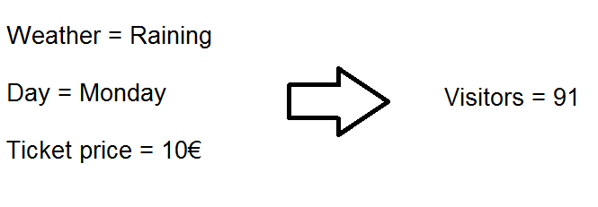
Problem. How to predict the number of visitors in an event?

Simple solution. Calculate the average from past events.

Machine learning solution. Take advantage of known event related variables when predicting number of visitors. These variables might be weather, day of week and ticket price. This makes the prediction more accurate than overall average.

Predicting by variables

#2 Clustering

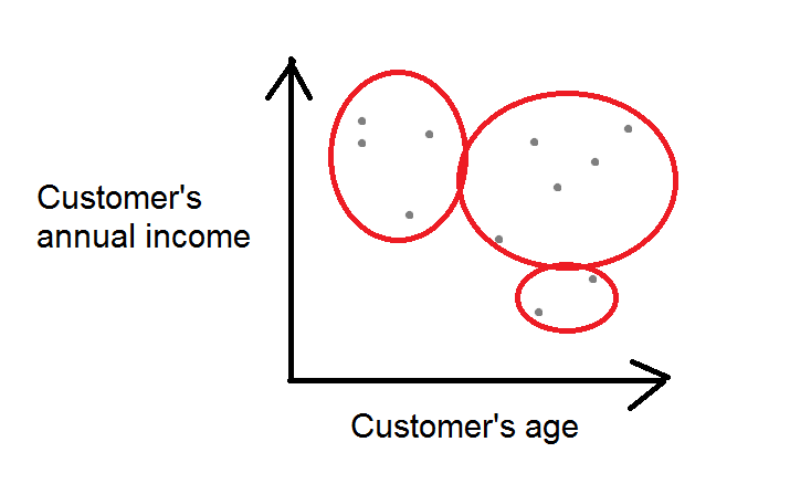
Problem. How to identify customer segments?

Simple solution. Make an educated guess by using fixed values.

Machine learning solution. The algorithm usually needs some initial parameters such as the number of clusters to identify. Segmentation process could be automated and standardized. The segmentation could be run once a day, week or month without any manual work. Another advantage is that there’s no need to set hard limits such as If customer’s annual income is more than 20 000€ and age more than 50, she’s in segment A. The algorithm will set these limits for you.

Machine learning clustering example

#3 Image recognition and classification

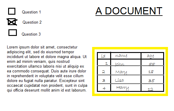
Problem. How to recognize objects, emotions or text from an image?

Simple solution. Do it manually.

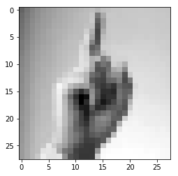
Machine learning solution. The algorithm has to be “trained” with already known cases to recognize which kind of pixel and color combinations means certain object. Image recognition could be used to identify data tables from hand written documents to transform the data to digital format. You could also detect other kind of objects such as a human face and take the analysis further by recognizing person’s emotions.

Image recognition example

A business problem: Online store deliveries

In the more detailed example, I will go through similar case than the #1: The process of predicting by variables as it is very common scenario in business analytics. Also many of the concepts can be used even in image recognition once the image pixels has been converted to tabular data.

Let’s imagine that we are running an online shop that orders nutrition supplements from a wholesaler and sells the products to consumers.

Machine learning on supply chain management

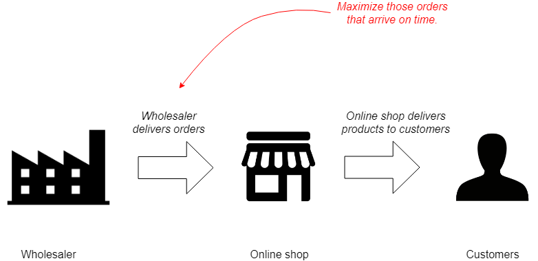
The online store wants to maximize those wholesale orders that will arrive on time. This will increase predictability and end user satisfaction, that will lead to bigger profits.

Sample data

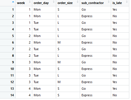
In the sample data a record corresponds to an order made for a wholesaler in the past. The first column is the week when the order has been made (week). Then there are the day of week (order_day), order batch size (order_size), sub contractor delivering the order (sub_contractor) and the info whether the delivery was late or not (is_late).

Sample data for machine learning

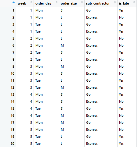
Usually collecting and cleaning the data is by far the most time consuming part. That has been already done in this example, so we can move to analysis. For example, maybe in the original data the size of order was the number of items, but for this case the variable has expressed in S (small), M (medium) or L (large).

There are dozens of predictive machine learning algorithms that work in a different way, but a typical situation is to create a table like this, where the last column is the variable that you want to predict. For historical data the predicted variable is known already. All or part of the other variables are predictor variables.

Result variable in sample data

Predicting from reports is not systematic

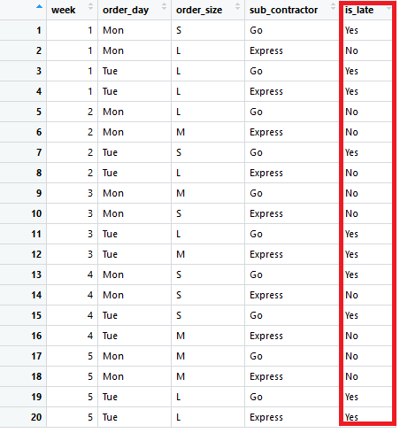
In traditional reporting you could analyze the rate of late arriving orders from previously introduced 20 rows of data by doing basic data aggregation and see how many percent of orders have arrived late on average for each variable combination.

Summary report

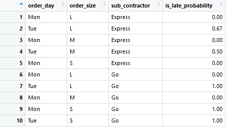
Using reports to forecast future is problematic, however. If there’s only one record for a combination such as Mon, L and Express in row 1, the probability is always 0 or 1, which can’t be true. The summary report also does not handle individual variables (columns) as independent entities, and that’s why there is no way of evaluating probability for previously non existing combinations such as Tue, M and Go.

And the most important part: There’s no way of evaluating how these insights fit into new wholesale orders.

Concept of training and testing in machine learning

The secret of predictive machine learning is to split the process in two phases:

  1. Training the model
  2. Testing the model

The purpose is, that after these two stages you should be confident whether your model works for the particular case or not.

For testing and training, the data has to be split in two parts: Training data and testing data. Let’s use a rule of thumb and take 70% of rows for training and 30% for testing. Note, that all the data is historical and thus the actual outcome for all records are known.

First 14 rows (70%) are for model training.

Training data

In the training phase the selected algorithm produces a model. Depending on the selected method, the model could be for example:

  • An algorithm.
  • A formula such as 2x+y+3z-1.
  • A lookup table.
  • A decision tree.
  • Any other kind of data structure.

The important thing is, that the produced model should be something that you can use to make predictions in the testing phase. The situation is very fruitful, as now you can make a prediction for each record in testing data with the model, but you can also see, what was the actual outcome for that observation.

The trained model will be tested with the last 6 rows (30%). Testing data

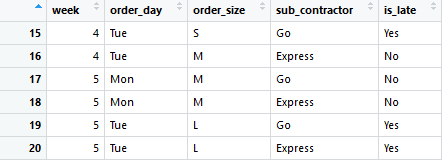
Selecting the machine learning algorithm

Normally you would pre-select multiple algorithms and train a model with each of them. The best performing one could be chosen after the testing phase. For simplicity, I selected just one for this example.

The algorithm is called naive bayesian classifier. I will extract the complicated name to its components.

Naive. The algorithm is naive or “stupid” as it doesn’t take in to account interactions between variables such as order_day and sub_contractor.

Bayesian. A field of statistics named after Thomas Bayes. The expectation is that everything can be predicted from historical observations.

Classifier. The predicted variable is_late is a categorical and not a number.

The naive bayesian classifier algorithm will be used to predict is_late when predictor variables are know beforehand: order_day, order_size and sub_contractor. All variables are expected to be categorical for naive bayes, and that is why it suits to out needs well.

Naive bayes classifier is quite simple algorithm and gives the same result every time when using the same data. It would be possible to explain the logic behind each predictions. In some cases, this is a very valuable.

The week column won’t be used for prediction and its purpose will be explained at the end of the next chapter.

Training and testing the model

Without going too deep in the details, you can run something like this in statistical programming language such as R:

model <- naiveBayes(is_late~order_day+order_size+sub_contractor, data=data.train)

And this kind of data will be stored in computers memory:

Naive bayes model output in R

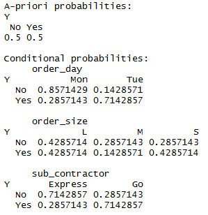
The point is not to learn inside out what these numbers mean, but to understand that this is the model and the software understands how to apply them to make predictions for new orders:

predictions <- predict(model, newdata=data.test)

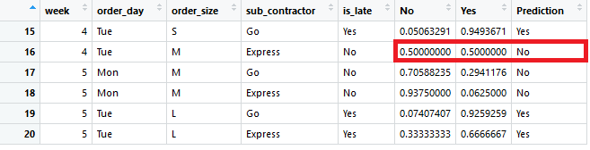
By doing some copy and paste operations, the predictions can be appended to testing data:

Naive bayes predictions

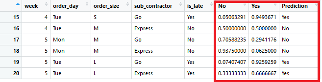
If the value in Yes column is more than 0.5, it means that the prediction for that order is to arrive late.

In our case the order of records matter: The model should be trained with observations that have occurred before the observations in test data. The number of week (`week`) is a helper column to order the data for train and test splitting.

Evaluating the goodness of the model

A good way to evaluate the performance of the model in this example is to calculate how many predictions we got correct. The actual value can be seen from is_latecolumn and the prediction from Prediction column.

Because I had the power to create the data for this example, all 6 predictions were correct. For the second record the probability for both being late and not being late was 50%. If this would have been interpreted as Yes, the prediction would have been incorrect, and the accuracy would have fallen to 83.3% or 5/6.

Naive bayes prediction 50-50

Evaluating the business benefit

So far we have:

  1. Identified a business problem.
  2. Combined and cleaned possibly relevant data.
  3. Selected a suitable algorithm.
  4. Trained a model.
  5. Tested the model with historical data.
  6. Evaluated the prediction accuracy.

Now it’s time to evaluate the business benefit.

We are confident, that our model is between 83.3% to 100% accurate for unseen observations, where only order day, order size and sub contractor are known before setting up the order. Let’s trust the mid point and say that accuracy is 91.7%.

You can count that in test data 3/6 or 50% of orders arrived late. Supposing that you would have used your trained machine learning model, you could have made the order only for those 3 or 4 deliveries that are predicted to arrive on time and a couple of additional orders that are not described in the test data.

In real world the situation would be more complex, but you get the idea that accuracy of 91.7% is more than 50%. With these numbers you are probably also able to estimate the impact in terms of money.

Implementing the model to daily work

Here are some ways to harness the solution for business.

Data study. Improve company’s process by experimenting the optimal order types.

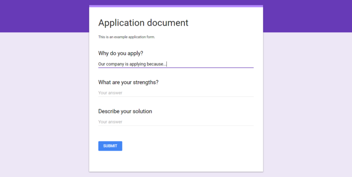
Calculator. Let employers enter the three predictor variables to a web calculator before placing the order to evaluate the risk of receiving products late.

Automated orders. Embed the calculation as part of the company’s IT infrastructure. The system can make the optimal orders automatically.

As time goes by, more historical orders can be used in training and testing. More data makes the model more reliable.

The model can be trained with the order data from past year once a day for example. Frequent training and limiting data only to latest observations doesn’t make machine literally learn, but rather this adjust the model to give the best guess for the given situation.

Summary

A predictive machine learning model offers a way to see the future with the expectation that the environment remains somewhat unchanged. The business decisions don’t need to be based on hunches and prediction methods can be evaluated systematically.

Thoughtfully chosen machine learning model is able to make optimal choices in routine tasks with much greater accuracy than humans. Machine learning makes it also possible to estimate the monetary impacts of decisions even before the actions has been taken.

Machine learning won’t replace traditional reporting nor it is in conflict with it. It is still valuable to know key performance indicators from past month or year.

Even though there are endless ways to do machine learning, predicting a single variable is a pretty safe place to start.

Data

week,order_day,order_size,sub_contractor,is_late
1,Mon,S,Go,Yes
1,Mon,L,Express,No
1,Tue,L,Go,Yes
1,Tue,L,Express,Yes
2,Mon,L,Go,No
2,Mon,M,Express,No
2,Tue,S,Go,Yes
2,Tue,L,Express,No
3,Mon,M,Go,No
3,Mon,S,Express,No
3,Tue,L,Go,Yes
3,Tue,M,Express,Yes
4,Mon,S,Go,Yes
4,Mon,S,Express,No
4,Tue,S,Go,Yes
4,Tue,M,Express,No
5,Mon,M,Go,No
5,Mon,M,Express,No
5,Tue,L,Go,Yes
5,Tue,L,Express,Yes

R Code

library(e1071)
library(plyr)
library(dplyr)

f.path <- 'C:/Users/user/folder/data.csv'
df <- read.csv(f.path, sep=",")
df

#Make a summery table
df.sum <- df
df.sum$is_late <- ifelse(df.sum$is_late=="Yes",1,0)
agg <- aggregate(df.sum[,'is_late'], list(df.sum$order_day, df.sum$order_size, df.sum$sub_contractor), mean)
names(agg) <- c("order_day","order_size","sub_contractor","is_late_probability")
agg$is_late_probability <- round(agg$is_late_probability,2)
agg

#Split to train and test data
data.train <- df[1:14, ]
data.train
data.test <- df[15:20, ]
data.test

#Count data by order size
table(data.train[1:14, 'order_day'], data.train[1:14, 'is_late'])
table(data.train[1:14, 'order_size'], data.train[1:14, 'is_late'])
table(data.train[1:14, 'sub_contractor'], data.train[1:14, 'is_late'])

#Fit naive bayes model
fit <- naiveBayes(is_late~order_day+order_size+sub_contractor, data=data.train)
fit

#Predict probabilites
probs <- predict(fit, data.test, type = "raw")
probs <- data.frame(probs)
probs

#Get more probable option
Prediction <- ifelse(probs$Yes>0.5,"Yes","No")

#Paste predicted probabilities to original data
data.test.new <- cbind(data.test, probs, Prediction)

#Prediction rate
sum(data.test.new$Prediction == data.test.new$is_late) / nrow(data.test.new)