Reading the genomic language of DNA using neural networks

Neural networks are powerful tools in natural language processing (NLP). In addition, they can also learn the language of DNA and help in genome annotation. Annotated genes, in turn, play a key role in finding the causes and developing treatments for many diseases.

April 1, 2022

Venla Viljamaa

I have been finishing my studies while working at Solita and got the opportunity to do my master’s thesis in the ivves.eu research program in which Solita is participating. The topic of my thesis consisted of language, genomics and neural networks, and this is a story of how they all fit into the same picture.

When I studied Data Science at the University of Helsinki, courses in NLP were my favorites. In NLP, algorithms are taught to read, generate, and understand language, in both written and spoken forms. The task is difficult because of the characteristics of the language: words and sentences can have many interpretations depending on the context. Therefore, the language is far from accurate calculations and rules where the algorithms are good at. Of course, such challenges only make NLP more attractive!

Neural networks

This is where neural networks and deep learning come into play. When a computational network is allowed to process a large amount of text over and over again, the properties of the language will gradually settle into place, forming a language model. A good model seems to “understand” the nuances of language, although the definition of understanding can be argued, well, another time. Anyways, these language models taught with neural networks can be used for a wide variety of NLP problems. One example would be classifying movie reviews as positive or negative based on the content of the text. We will see later how the movie reviews can be used as a metaphor for genes.

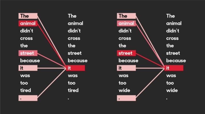
In recent years, a neural network architecture called transformers has been widely used in NLP. It utilizes a method called attention, which is said to pay attention to emphases and connections of the text (see the figure below). This plays a key role in building the linguistic “understanding” for the model. Examples of famous transformers (other than Bumblebee et al.) include Google’s BERT and OpenAI’s GPT-3. Both are language models, but transformers are, well, transformable and can also be used with inputs other than natural language.

An example of how transformers self-attention “sees” the connections in a sentence. The difference of the last word completely changes what the word “it” most refers to.

DNA-language

And here DNA and genomes come into the picture (also literally in the picture below). You see, DNA has its own grammar, semantics, and other linguistic properties. At its simplest, genes can be thought of as positive movie reviews, and non-coding sequences between genes as negative reviews. However, because the genomes of organisms are part of nature, genes are a little more complex in reality. But this is just one more thing that language and genomics have in common: the rules do not always apply and there is room for interpretation.

Simplification of a genome and a gene. Genomic data is a long sequence of characters A, T, C, and G representing four nucleotide types. Genes are coding parts of the genome. At their simplest, they consist of start and end points and the characters between them.

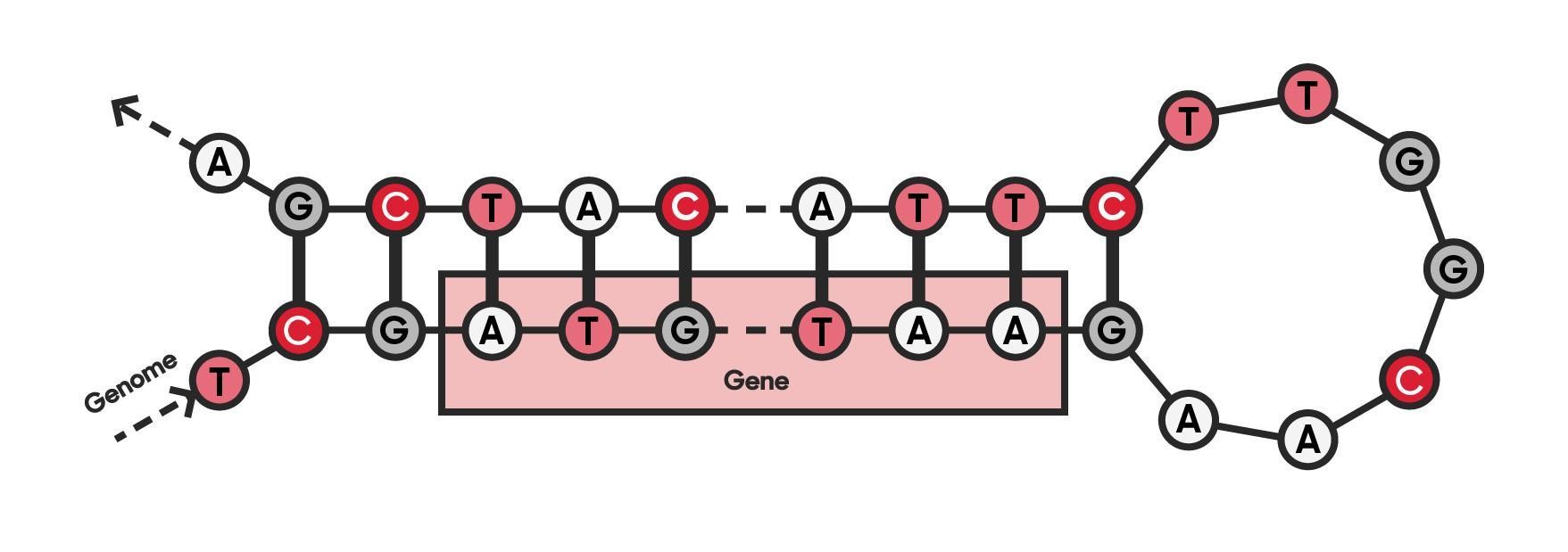
Since both text and genomic data consist of letters, it is relatively straightforward to teach the transformer model with DNA sequences instead of text. Like the classification of movie reviews in an NLP-model, the DNA-model can be taught to identify different parts of the genome, such as genes. In this way, the model gains the understanding of the language of DNA.

In my thesis, I used DNABERT, a transformer model that has been pre-trained with a great amount of genomic data. I did my experiments with one of the most widely known genomes, E. coli bacterium, and fine-tuned the model to predict its gene locations.

Example of my experiments: the Receiver operating characteristic (ROC) curves helped me to find the most optimal input length for the genome data. Around 100 characters led to the highest curve and thus the best results, whilst 10 was obviously too short and 500 too long.

After finding the most optimal settings and network parameters, the results clearly showed the potential. Accuracy of 90.15% shows that the model makes “wise” decisions instead of just guessing the locations of the genes. Therefore the method has potential to assist in the basic task of bioinformatics: new genomes are sequenced at a rapid pace, but their annotation is slower and more laborious. Annotated genes are used, for example, to study the causes of diseases and to develop treatments tailored to them.

There are also other methods for finding genes and other markers in DNA sequences, but neural networks have some advantages over more traditional statistics and rule based systems. Rather than human expertise in genomics, the neural network based method relies on the knowledge gathered by the network itself, using a large amount of genomic data. This saves time and expert hours in the implementation of the neural network. The use of the pre-trained general DNA language model is also environmentally friendly. Such a model can be fine-tuned with the task-specific data and settings in just a few iterations, saving computational resources and energy.

There is a lot of potential in further developing the link between transformer networks and DNA to study what else the genome language has to tell us about the life around us. Could this technology contribute to the understanding of genetic traits, the study of evolution, the development of medicine or vaccines? These questions are closely related to the healthcare field, in which Solita has strong expertise, including in research. If you are interested in this type of research, I and other Solita experts will be happy to tell you more!

Venla Viljamaa (Data Scientist) venla.viljamaa@solita.fi linkedin.com/in/venlav/

FastText in a text classification project

In this blog I describe how we did text classification for funding applications with FastText package.

January 27, 2019

Mikael Ahonen Data Scientist

Describing the business need for text mining

Companies applied funding with this kind of form.

Application form could have been something like this. The form is a simplified example.

The documents were classified in a several categories by the application handler in the process management software.

The handler classified the application document in several categories base on application texts. — The human handler classified the application to categories such as Business development, Agriculture and Digitalization.

The manual process was not only time consuming, but also frustrating. Reporting was the primary reason for the classification.

Text data is often the most sensitive data

We had two primary ways of getting data.

Customer’s software was developed by Solita’s team. This made it easy to access the SQL database of the testing environment. As a result, we had all numerical and structured data in our hands. Numerical data was useful for application risk prediction, but we needed text data for document classification.

The text data was encrypted in the test database. This meant that we needed a way to securely import the plain language text data from the production SQL database.

There is a good reason why the access to text data should not be easy. Text data might contain sensitive information such as personal data or business secrets.

Selecting FastText as our text mining tool

My personal experience from text mining and classification was very thin. After discussions with the team we decided to go with the FastText package. It has been designed for simple text classification by Facebook.

FastText is quite easy command line tool for both supervised and unsupervised learning. We used a python package which apparently don’t support all original features such as nearest neighbor prediction [link].

For supervised prediction you create individual text files for training and testing data [link]. After files are created, training the neural network behind FastText takes just a few lines of code. We used the supervised method to classify the applications.

Example from FastText supervised tutorial data. FastText training data has labels at the beginning of each line followed by the actual text. — FastText training data has labels at the beginning of each line followed by the actual text.

For unsupervised analysis you can just dump a bunch of text to a file to create word vectors [link]. Word vectors are useful for finding words similar to each other.

While English has either singular or plural format such as dog or dogs, Finnish language has koira, koirat, koirani, koiranne, koirienne, koirilatammekohan… There are literally tens of variations for each word. FastText is especially great for languages like Finnish where suffixes at the end of each word vary depending on the context. This is because in addition of creating features from word counts FastText can also take into account combinations of words as well as sub-word character sequences.

A model per category using a document as an observation

Each application had multiple text fields and multiple categories to automatically predict. How to approach the complex problem?

In database the there was individual row for each combination of application and text field. — In database the there was a row for each combination of application and text field.

We decided to bundle all applicable text fields from the applications together. Another option would have been to make predictions for each combination of application and text field, and then select the class with most “votes” from text field predictions.

We combined all answers to a single string and make one prediction per application. — We combined all answers to a single string and did one prediction per application.

We left out text fields such as team description. Those fields did not bring significant information for the classification.

Trying to understand the labeling principles of FastText made us scratch our heads. The initial idea was to create a single classification model. That model would have included all related labels in a single training row.

In theory this could lead to a situation where all top predictions are from the same category such as Digitalization. As we wanted to get the most probable prediction from each category, we decided to train individual model per category (Business development, Agriculture and Digitalization).

FastText supervised algorithm accuracy

The labels inside categories were unequally balanced. Some categories had even tens of labels with very few observations.

Example of label count shares for Digitalization category.

Class imbalance meant that prediction accuracy reached 50% to 90% for some categories by simply guessing the most frequent label. We took this as our base line.

Eventually our model-per-category-strategy produced a few percentage units higher accuracies than choosing the most common label. This only happened after we decided to return the weakest predictions back to manual processing. The probability of prediction’s correctness was automatically given by FastText.

In our case it was enough to beat the naive strategy of choosing the most common label.

The prediction ability of FastText increases when applications with low prediction probability are returned to manual classification. This decreases the number of applications getting automated prediction.

Summarizing the FastText classification experiment

Apparently the application handlers don’t pay too much attention about which label they choose. This made us question the whole process. What is the value of reports that are based on application handler’s hunch? And if the labeling criteria are not uniform, how could a machine find any patterns?

Let’s say there are 2000 annual applications. One of the labels gets selected 30 times per year. Binomial probability calculation reveals that 95% confidence interval for 30 labels is actually from 20 to 40. A decision maker might think that a series of 20, 30 and 40 during a three year range indicates ascending trend for the label. But in reality, it’s just a matter of random variation. In one of the categories 15 out of 20 labels had this few or less observations.

FastText favored more common labels as it increased the overall accuracy. This came with the cost that some labels never got predictions.

When the solution has ran in production for a while, it is time to see if the handlers ever make the effort to correct the machine’s initial recommendation. If not, some labels will never end up to the reports.

There are endless number of solutions to automate such document classification. In our project the fast testing cycle to try different approaches was the key. The goal was not to make perfect, but improve the existing situation.

Whatever the prediction accuracy will be, this kind of text mining experiment provides valuable information for the organization.

Why are deep learning models so popular?

Deep learning (i.e. big neural networks) plays a central role in the ongoing boom of artificial intelligence and data science. Last year, a partly neural network based AI beat a human grandmaster for the first time in Go, a complex board game. Judging by the hype, it feels like deep neural networks can be found in every other state-of-the-art AI solution.

January 2, 2019

Jesse Vuorinen

In practice they have their downsides, but although they are not the be-all-end-all of machine learning algorithms, neural networks are versatile and useful. In our client projects, we have leveraged deep learning in image recognition and multivariate time series forecasting tasks, for example. What qualities make neural networks efficient?

On a high level, a neural network (and most other supervised machine learning algorithms) can be seen as a device that takes in numerical inputs and spits out numerical outputs.

When the model is built, the general structure of what is inside the device, as well as the structure of its inputs and outputs, is specified. At this point, the model already “works” in the sense that it can take inputs to produce outputs, but the results are random.

Then, the model is trained by continuously feeding it with actual data, that is, correct answers to the problem at hand. During this training process the parameters of the model (the bolts and cogs inside the device) are adjusted in very small increments. In time, the algorithm converges and learns the relationships in the training data. In the end, the model learns how to map input data to outputs using a similar logic that underlies the training data it was fed. After training, the model can be used to make predictions based on new input data, something that the model has not seen before.

What goes in, what goes out?

The inputs to the device could be virtually anything that can be represented as arrays of numbers: images, time series data, videos, free text articles after being transformed into numerical representations, you name it. The outputs can also take various shapes.

The output could be a single number, say a weather forecast on a given hour. Or it could be an array of several figures, like the pixel coordinates of an identified suspected cancer in an x-ray image received as input.

The end result does not even have to be numeric, even though a neural network only crunches numbers. For example, the network can produce an array of likelihood estimates that are converted into a categorical classification in the end.

Given a picture, the model could say it is a cat with 80 % certainty, a dog with 15 % certainty or a car with 5% certainty. Although almost anything can be represented in numerical format in some manner, deciding how the numerical representations of the inputs and outputs are actually done is usually not easy. This preprocessing step is an important part of the data science workflow.

Anatomy of a neural network

In the case of neural networks, what is inside the device is a large amount of interconnected simple processing units called neurons. A neuron takes a number, squeezes it through some non-linear function and then outputs the result. In a deep neural network, the neurons are organized into layers that succeed each other. The input signal is first sent to the first layer of neurons, which send their outputs to all the neurons in the next layer. This process continues layer after layer until the output layer is reached. The construct is inspired by biological neurons, the main components of the central nervous system.

The connections between neurons are also given so called weights, which are basically little valves that determine how much of each input the unit propagates up the network. Adjusting these weights is what actually happens during the training process and what allows neural networks to fit specific problems. A deep neural network could contain millions of weights, so the good news is that adjusting the weights can be automated efficiently (using backpropagation and gradient descent methods).

Advantages of neural networks

The idea of training a machine to transform numerical representations of inputs to outputs applies to most machine learning models, so what makes neural networks work special? Three reasons come to mind.

First, the structure of a neural network is specified only very broadly before the model is trained, which gives a lot of room for the model to adjust during training.

In statistical terms, large neural networks can be thought of as being somewhere in between parametric and nonparametric models. In a parametric model, for instance a traditional regression, the number of parameters in the model is strictly determined before fitting the model. In a nonparametric model, the model structure is determined more broadly, and the training process can adjust the number of parameters as well as their values. Thus, in a nonparametric model, there is more freedom for the model structure to adjust to the problem being solved. In neural networks, the number of parameters (weights) is strictly determined beforehand, which would imply that they are parametric models. However, the number of weights can be enormous and the training process could allow many of the weights to zero out, effectively blocking certain paths through the network. For these reasons, deep and broad neural networks resemble nonparametric models in practice. The nonparametric nature gives neural networks structural freedom to adapt to many kinds of problems.

Second, since neural networks consist of chained little functions that perform nonlinear transformations at each step, they are inherently nonlinear models.

This allows them to model many problems better since many real-world relationships are nonlinear. (For example, the area of a square shaped field increases exponentially instead of linearly as its width increases.)

Third, the vanilla version of a neural network that has been discussed so far can be adjusted to make it a better fit to certain problems.

Convolutional neural networks, for example, are good at making broad abstractions from very detailed inputs and work especially well for image recognition problems. In recurrent neural networks, the neuron layers have feedback loops, which essentially means that the network is able to remember previous inputs. This trait makes them a good fit for time series forecasting and natural language processing.

Advanced deep learning models – the ones that are used in solutions that are able to beat humans in complex games or drive vehicles – combine these basic architectures. For instance, the model could begin with convolutional layers that are good at abstracting information. This network could be followed by a recurrent network that has a memory and the ability to learn sequential and spatial relationships. Finally, a regular fully connected layer could produce the final output.

The downsides

If deep learning is so powerful, then why don’t we dump all other machine learning algorithms in their favor? One of the biggest caveats of neural networks is the fact that they are black boxes: it is usually impossible to intuitively explain why a neural network has given a certain prediction. Sometimes, the intermediate outputs that the neurons produce can be analyzed and explained, but many times this is not the case. Other algorithms, such as traditional linear models or tree-based models like random forest, can usually be analyzed and explained better.

Another downside is that neural networks need large amounts of training data and can take a long time to learn. This was a huge problem in the past but has been mitigated somewhat by technological advancement. One of the reasons for the surge in deep learning’s popularity can be attributed to improvements in GPU computational power and the advancements of cloud computing. Today, it is possible to train complex deep learning models in a matter of hours, not weeks.

How to get started?

Even though they are technically formidable when you dive into details, neural networks are not that hard to experiment with. A good way to get your hands dirty, if you know Python or R, is to first google and follow through hands-on coding tutorials, like this one. It is also a good idea to register into www.kaggle.com and build a neural network solution to one of the simpler problems, say, “Titanic: Machine Learning from Disaster”.

Once familiar with the basics, try something a little more advanced by following along these inspiring blog posts, for example: