AWS forecast service modelling Electricity consumption

Timeseries forecasting often requires significant mathematical knowledge and domain experience. This area of machine learning is often only accessible to experts, however, Amazon Forecast provides a simple and intuitive interface for creating complex machine learning models.

Timeseries forecasting is the process of looking at historical data to make predictions about the future. Companies can use these predictions to extract actionable insights that drive innovation. Often, the mechanisms behind the transformation of raw data into business value is a mystery to non-specialists. This is because timeseries forecasting requires expert knowledge of algorithms and mathematical concepts such as calculus. This is a domain reserved for the highly trained specialists, often not accessible to the average user. However, with the development of Amazon Forecast this could be changing.

Amazon Forecast is a fully managed service that simplifies the process of timeseries forecasting by hiding the inner complexity from the users. The user simply has to provide an input data, Forecast then automatically applies and selects the most optimal machine learning algorithm for the data to generate accurate predictions with little to no user intervention. This system is known as a ‘Black Box Method’, where a user can conduct complex modelling tasks without worrying about the low-level calculus and algorithms.

This movement of machine learning from experts to general users marks a significant paradigm shift known as AutoML (Automatic Machine Learning).

Within this blog Amazon Forecast will be explored from the perspective of a non-expert general user to assess how easy it is to get started producing accurate future predictions. In other words, can someone who is not a professional machine learning specialist produce professional models?

What we will predict

In this hypothetical scenario we work for an electricity provider and have been tasked with building a model to predict future electricity consumption for our customers. The input data we have been provided contains measurements for electricity consumption (Kw) every hour for 370 different clients from January 2014 – November 2014. This dataset contains 2,707,661 observations. We will build a model to predict the electricity consumption for the 1st of October 2014, so 24 hours into the future for every customer.

Creating the electricity forecast

 Unfortunately, Forecast is not able to clean and prepare your input data, you must ensure the data is prepared beforehand. This is the only technical step that is required in the forecasting process. In this instance, we prepare the dataset to match the schema requirements of Forecast as shown in the table below. Once prepared the data must be stored in an S3 as a CSV.


Client Timestamp Consumption
Client_1 2014-01-01 01:00:00 23.64
Client_0 2014-0101 02:00:00 9.64


As a general user we can achieve everything we need to generate a forecast within the Forecast Console. This is a no-code user interface in the form of a Dashboard. Within this dashboard we can manage all aspects of the forecasting process, this process is implemented in 3 easy steps:

  1.   First, you import your Target time series data. This is simply the process of telling Forecast where to find your prepared data in S3 and how to read the contents (schema).
  2.       Next, you use this Target time series to create a predictor. A predictor is a Forecast model trained on your timeseries. This is where the AutoML aspects of Forecast are truly utilised. When training a predictor in a typical timeseries forecast, the user would need to identify the optimal algorithm to train the model and then optimise this model. Within Forecast, all of these steps are done automatically using back testing. Back testing is the process of retaining a portion of the training data to train on all the algorithms to find the best fit.
  3.       Finally, with the model trained, we can generate a forecast. This is as simple as a few clicks on the dashboard. This will generate future predictions of energy consumption for every hour for every customer.

Now, with zero coding or expert input we have generated an advanced forecast utilising cutting-edge deep learning machine learning algorithm. If it appears very simple, that’s because it is. The dashboard was designed to be simple and easy to use. For more advanced users Python can be used to connect to Forecast where you gain significantly more control over the process. But as a general user such control is not necessary.

Visualise and export the electricity consumption predictions

For this section we will visualise the forecasted predictions for customer 339, found in the graph below. As we actually have the real observed values for the 1st of October 2014, we can compare our predictions with the actual observed electricity consumption.

In the graph the darker blue line represents the real values. We can also see a red line and a light blue area. This blue area is known as the 80% confidence interval, indicating that we are 80% confident that the real value will lie somewhere within this area. The red line, p50 value (median forecast) can be considered as an indication of the ‘most likely outcome’.

As we can see, our forecast appears to be very accurate in predicting the electricity consumption for this customer, with the predicted values closely following the observed values. In practice, these forecasts could be used in a variety of ways. For example, we could share this forecast with the customer, who can then adjust their consumption patterns to reduce energy usage during peak hours and thus lower energy bills. For the energy provider, these forecasts could be used in load management and capacity planning.

Conclusion

The main purpose of Forecast and AutoML is to allow non-experts to develop machine learning models without the required expertise. AutoML also enables experienced data scientists by reducing time spent optimising models. Forecast achieves both, as I, a non-expert, was able to develop an advanced forecasting model without any interaction with the complex underlying mechanisms. It is clear Forecast extends the power of time series forecasting to non-technical experts, empowering them to make informed decisions from machine learning insights.

AWS re:Invent 2022 re:Cap

AWS re:Invent is the biggest AWS conference in the world with over 50,000 participants and 2600 sessions to choose from over five days. This blog is a recap of the event and the sessions that I attended to give you an idea of what happens during the hectic week in Las Vegas.

After two years of virtual events and uncertainty in travel restrictions, this year it finally looked possible to attend the biggest AWS event on-site too, so I definitely wanted to take the opportunity to head to Las Vegas once again. I have been to two AWS conferences before (re:Invent in 2018 and re:Inforce in 2019), so I already had some idea of what to expect from the hectic week. You can read more about what to expect and tips and tricks for attending from the previous blog posts, as most of them applied this year too and the conference itself hasn’t changed that much from previous years. In this blog post, I’m going to summarize all the different sessions that I attended during the week to give you an idea of what’s happening during this massive and long event.

Pre-planning and scheduling

re:Invent is always a huge conference and this year made no exception. With over 50,000 participants and 2600 sessions to choose from over five days, there’s a lot of content for almost everything AWS related. With the massive scale of the conference comes some challenges related to finding relevant content. There are different types of sessions available, with breakout sessions being lecture-type presentations that will be published to YouTube later on. Therefore, I tried to focus on reserving seats to more interactive, Q&A focused Chalk Talks and hands-on workshops, as those are only available at the event itself.

This year, reserving seats to the sessions went pretty smoothly, but once again the calendar and session finder were quite lacking in helpful features that would make the process a lot easier. For example, you can’t easily search for sessions that would fit your calendar at the location your previous session ended, but have to go through the session list manually with some basic filters. Also, since there are many different venues and traveling between venues takes a lot of time, you would want to minimize the amount of venues per day, but for some reason the sessions I wanted to go to were scattered all over the campus. So initially, my calendar looked pretty unrealistic, as sessions were in multiple different locations throughout the days. Therefore I ended up just focusing on a couple of longer workshops per day, and favoriting a bunch of sessions in the same location as the previous or next session. This way, I could easily have a “Plan B” or even a “Plan C” when trying to find a walk-up spot for some of the sessions.

However, this meant that my calendar for the week ended up looking like this:

Overall, the scheduling experience was still a bit lacking compared to the excellent quality of the conference otherwise. But at least this time in the end I managed to get in to pretty much all of the sessions I wanted to, and the schedule worked out pretty well in practice too, as you could utilize the free time between sessions with all the nice things happening around (content hub, labs, jam lounge) and just walking around the huge expo area (talking to AWS staff, vendors and also collecting some nice swag)

Notes from the sessions

Here are some short recaps on the different sessions that I attended during the week.

Day 0 – Sunday

The whole Solita crew attending the event started the journey with the same flight, but after some unfortunate flight delays, we were split to different connecting flights in Dallas and finally arrived to Las Vegas in late Saturday night after 22 hours of traveling and a lot of waiting.

For some reason, the traditional Midnight Madness event with the first announcements was not held this year, so Sunday was quite relaxed with some strolling around while trying to deal with jet lag. Badge and hoodie pickup points opened on Sunday, so that was pretty much the only official agenda for the day. In the evening we had dinner with the whole Solita crew attending the event this year.

Day 1 – Monday

Hackathon: GHJ301-R – AWS GameDay: The New Frontier

Day one started early at 8:30 AM with one of the most interesting sessions available – the GameDay Hackathon where teams of four compete against each other in a gamified learning experience. Because there was no reserved seating available for this year’s GameDay sessions, I wanted to make sure to get there in time. And due to some jet lag, a brisk morning walk was also a good way to wake up. In the end, I was there way too early as there wasn’t a huge queue to get in like I had thought and the room didn’t even get full.

The concept of GameDay was a bit different this year, as there were independent quests and challenges instead of one unifying challenge. In 2018, the theme was microservices and trying to keep the services up and running while something unexpected occurred. That required a bit more teamwork, as now you could just focus on working on one challenge at a time individually.

There were also some bonus quests added during the session, and even Jeff Barr made a quick visit on stage announcing a trivia bonus quest. In the end, our team finished 10th out of roughly 40 participating teams, but we could’ve had a lot more points if we had done some of the challenges in a different order, as there were some that were generating a lot more points based on the time they were completed.

Overall, it was a fun learning experience once again, as you get to solve some puzzles and try new services in a more hands-on way than in a workshop. 

Workshop: AIM312-R – Build a custom recommendation engine in 2 hours with Amazon Personalize

Next up was a 2 hour workshop focused around recommendations using Amazon Personalize. I have previously tinkered with the service right when it launched, and it was a bit limited in features back then. Over the years they have added some new things like promotions, campaigns and metrics, but if you are trying to do anything more complicated, you might quickly run into the limits of the service.

The title of the workshop was a bit misleading, since the actual model used for recommendations was already pre-built and would take way longer than 2 hours to complete even with the small dataset that was used in the workshop.

Session: BOA304 – Building a product review classifier with transfer learning

I had scheduled a second workshop for the afternoon but it would have been on the other side of the campus, so I opted for staying near Venetian so that I could visit the Expo area too. Found a breakout session with an interesting topic so I decided to join it as a walk-up. The very quick 20 minute session was about using a pre-built model from Hugging Face in Sagemaker and doing some transfer learning for building a simple helpful/not helpful classifier for Amazon.com product reviews.

Chalk Talk: DAT301 – Use graphs to perform fraud analysis with Amazon Neptune and Neptune ML

I also managed to get in a chalk talk as a walk-up without any queueing(!). Apparently graph databases are still not that widely used. It was an interesting session though, and with chalk talks you get a lot more opportunities for interacting with and asking questions from the presenters. 

Neptune ML seems like a pretty nice wrapper for Sagemaker, but it looked like you needed to use property graphs (Gremlin or openCypher) instead of RDF (SPARQL). The upcoming Graph Explorer looked nice compared to the current very limited visualization tools available using Neptune Notebooks. Some pretty good conversation sparked from questions from the audience regarding data modeling in graph databases.

After the sessions on Monday evening, AWS Nordics hosted a welcoming reception in one of the restaurants located inside Venetian, the main conference hotel. It was quite packed, but it was nice to meet new people from other companies in Finland.

Day 2 – Tuesday

Keynote: Adam Selipsky’s keynote

To save some time on traveling between venues and waiting in queues, I opted to watch the Tuesday morning’s main keynote from an overflow space located at my hotel. Loads of new announcements and customer cases were shared once again. The biggest data related announcements were probably OpenSearch Serverless, the “zero-ETL” integration of Athena and Redshift, general availability of Redshift streaming ingestion from Spark, and Datazone, a new data catalog and governance tool which I hoped to learn more about in a new launch session, but unfortunately there weren’t any available and even the blog post was quite vague on details.

Workshop: LFS303 – Finding data in a life science data mesh

The first workshop on Tuesday focused on creating a data mesh setup with multiple different health care data sets in S3 that were cataloged using Lake Formation and crawled using Glue. Information about the data sets was then converted into RDF Triples and loaded into Amazon Neptune so that graph traversal queries can be done and medical codes can be combined with the hierarchical medical code ontology data set to create a knowledge graph where you can find out the data sets where the data you are looking for is located in, using differently formatted medical codes. Then you can use Lake Formation to provide fine grained access to the data and Athena to query the actual data.

This was a pretty good and informative workshop with some similarities to one use case in my current project too (Neptune and hierarchical ontologies), and I learned something new from Lake Formation which I hadn’t used before too.

Workshop: DAT310-R – Develop event-driven applications using Amazon Aurora Serverless v2

The agenda for the second workshop of Tuesday was building a simple voting web application using serverless components (Aurora Serverless, Lambda, API Gateway and Cloudfront) and auto-scaling, with authentication using Cognito. The use case was quite basic, so nothing too special was done in this workshop, but it was still nice to see how quickly Aurora is able to auto-scale when the load increases or decreases, while latencies to the web application remain low.

Session: CMP314 – How Stable Diffusion was built: Tips and tricks to train large AI models

There wasn’t any space for two chalk talks that I tried to join as a walk up (without reservation), so instead I went to listen to a session on how the text-to-image ML model Stable Diffusion was trained instead. It was fun to hear from the challenges that training that massive of a model has and the infrastructure around it, even though this massive ML model training is probably something I won’t be doing anytime soon.

After the sessions on Tuesday night there were some sponsored restaurant reception events at the venues, and in addition to that I attended an event hosted by Databricks at Topgolf. It was a fun experience to try some rusty golf swings on a gamified driving range while meeting new people and discussing what they are doing using AWS services.

Day 3 – Wednesday

Workshop: BOA325-R – Building a serverless Apache Kafka data pipeline

On Wednesday morning Swami Sivasubramanian hosted a keynote focusing on data & machine learning. I had booked a workshop at the same time, so I tried to follow the keynote while waiting for the workshop to start. Some new features for existing products were announced, for example Spark support for Athena and Geospatial ML for Sagemaker.

The actual workshop was focused on building a quite simple data pipeline with a Fargate task simulating generating clickstream events, sending them to Kafka which triggered a Lambda to convert the events to a CSV format and upload that to S3. Converted files were then visualized in QuickSight.

Workshop: ANT312 – Streaming ingestion and ML predictions with Amazon Redshift

Second workshop of the day focused on the new-ish streaming ingestion and ML features of Redshift. First streaming data was loaded from Kinesis to Redshift using the new Streaming Ingestion feature where you don’t need to use Firehose and S3 but you can just define the Kinesis stream as an external schema and create a materialized view for the stream data. Kafka (MSK) streams were supported too. After configuring the streaming data as a materialized view and loading some historical data, Redshift ML was used to build a XGBoost binary classification model for finding fraudulent transactions directly from the stream based on history data. Quicksight was then used for visualizing the data and to create a dashboard for the fraudulent transactions.

Also had some extra time between workshops and didn’t have any room to join nearby workshops or chalk talks as a walk-in, so went to the overflow content hub to briefly listen to some on-going sessions regarding EKS and Well-Architected Framework.

Workshop: ANT310-R – Build a data mesh with AWS Lake Formation and AWS Glue

Third and last workshop of the day focused on creating a quite complex data mesh setup based on AWS Analytics Reference Architecture using Lake Formation, Glue, CDK and Athena. Basically it was about sharing your own data set to a centrally governed data catalog with some Named/Tag based access control, and then accessing data from other accounts in the data catalog and combining them in queries using Athena.

Day 4 – Thursday

Hackathon: GHJ206-R – AWS Jam: Data & Analytics

Thursday morning started with some jamming instead of the Werner Vogels keynote that was happening at the same time. I glanced through the announcements from the keynote afterwards, and at least Eventbridge Pipes and Application Composer looked like interesting announcements.

This year there were also separate Jam events in addition to the Jam Lounge at the Expo area, where you could again complete different challenges during the whole week. The separate Jam events were only three hours long and teams of four competed in completing challenges while collecting points, similarly to this year’s GameDay. The Jam event I was most interested in was focusing on Data & Analytics, with challenges ranging from using Amazon Rekognition for facial image recognition to creating real time data analytics pipeline using Kinesis Data Streams and Kinesis Data Analytics Studio.

Luckily we got some very talented people in our team and we managed to complete almost all of the challenges. In the end, we finished first out of 50 participating teams and won the jam, and got some nice prizes for the effort too. It was a close competition and we managed to climb to the first position only in the very last minutes. Overall it was again an intense but fun experience and I managed to learn some new things regarding Sagemaker and Kinesis.

Session: DAT328 – Enabling operational analytics with Amazon Aurora and Amazon Redshift

There were a couple of new launch sessions added to the catalog after the keynotes, and this time I managed to get a seat in a couple of them. This session focused on the “zero-ETL” linking of Amazon Aurora and Amazon Redshift, where Aurora data will be automatically synced to Redshift without having to write any code. Basically you first needed to configure the integration using the Aurora console, and after that a new database was added to Redshift. After that, an initial export was done, CDC logging was enabled in Aurora and future changes will be synced automatically to Redshift to the newly created database. Currently the feature only supports Aurora MySQL and is available in preview only. It also seemed to lack any features for example for filtering the synchronization to use only a specific table or multiple tables in Aurora.

Workshop: CON402-R – Concepts to take your Kubernetes operations and scale to the next level

Last workshop of the week was focused on some best practices for scaling, security and observability inside EKS. It’s still quite cumbersome and slow to set up and the developer experience for Kubernetes still isn’t great. Cluster autoscaling was done using Karpenter, security was improved using IAM role based access control and pod level security, observability was done using CloudWatch Container Insights, OpenTelemetry and X-Ray.

Chalk talk: AIM341-R – Transforming responsible AI from theory into practice

Last chalk talk of the day was an interactive discussion on how to build responsible ML models, which aspects to take into account and how to make ML models more explainable. Would have liked to see more concrete examples on how to take all those things into account at the model level.

Thursday night was the re:Play night. Before the main event, there was also a AWS Certified Reception pre-party held at at a local bowling alley with also other fun and games. The main event took place at the nearby Festival Grounds and it was a great night filled with music, good food, drinks and meeting up with colleagues and new people, with Martin Garrix and Thievery Corporation headlining the two live music stages. This time it took quite a lot of time to get in and out of the party, as wait times for shuttles were long and traffic was slow. 

Day 5 – Friday

Session: ARC313-R -Building modern data architectures on AWS

Even though most of the content at re:Invent happens between Monday and Thursday, there were still a couple of sessions held on Friday morning too. This session was quite an information dump showcasing the multiple different AWS resources available for reference architectures for different data use cases and data platforms. Focused on six different layers: ingestion, storage, cataloging, processing, consumption and governance, with providing reference architectures and services to use for each of those. What also became clear with this session is that AWS has quite a lot of overlapping services these days, and the ones you should use depend quite a lot on your use case.

Session: API206 – Amazon EventBridge Pipes simplifies connecting event-driven services

Last session of the week was a brief overview and demo on the new EventBridge Pipes feature announced at Werner’s keynote on Thursday. It provides a simple way to integrate different AWS services without writing extra code. It looks pretty easy to use for simple use cases, where you might need to do some filtering for Kinesis streams or call a Lambda for transforming data, and then passing on the data to another service like SQS. They wanted it to work kind of like UNIX pipes, but for AWS services.

Conclusions

Overall, re:Invent 2022 was again a great learning experience and an exhausting but rewarding week. The days were long but there’s so much new to learn and things happening all the time that the week just flew by very quickly. It was great to finally attend a large conference after a couple of years of online-only events which just don’t work the same way in terms of learning and networking in my opinion. You could easily spend the whole week just in the expo area talking to different vendors and AWS staff, and still learn a lot without even attending the sessions.

Even though the conference is massive in its scale, almost everything worked smoothly without any major issues. I’d still agree with pretty much all of the conclusions from my previous blog post again, and re:Invent is definitely a conference worth attending even though it is a pretty big investment timewise. Hopefully I’ll get the chance to attend it again some time in the future.

Also keep an eye out for upcoming re:Invent blog posts in our Dev and Cloud blogs too.


A Beginner’s Guide to AutoML

In a world driven by data, Machine Learning plays the most central role. Not everyone has the knowledge and skills required to work with Machine Learning. Moreover, the creation of Machine Learning models requires a sequence of complex tasks that need to be handled by experts.

Automated Machine Learning (AutoML) is a concept that provides the means to utilise existing data and create models for non-Machine Learning experts. In addition to that, AutoML provides Machine Learning (ML) professionals ways to develop and use effective models without spending time on tasks such as data cleaning and preprocessing, feature engineering, model selection, hyperparameter tuning, etc.

Before we move any further, it is important to note that AutoML is not some system that has been developed by a single entity. Several organisations have developed their own AutoML packages. These packages cover a broad area, and targets people at different skill levels.

In this blog, we will cover low-code approaches to AutoML that require very little knowledge about ML. There are AutoML systems that are available in the form of Python packages that we will cover in the future.

At the simplest level, both AWS and Google have introduced Amazon Sagemaker and Cloud AutoML, which are low-code PAAS solutions for AutoML. These cloud solutions are capable of automatically building effective ML models. The models can then be deployed and utilised as needed.

Data

In most cases, a person working with the platform doesn’t even need to know much about the dataset they want to analyse. The work carried out here is as simple as uploading a CSV file and generating a model. We will take a look at Amazon Sagemaker as an example. However, the process is similar in other existing cloud offerings.

With Sagemaker, we can upload our dataset to an S3 bucket and tell our model that we want to be working with that dataset. This is achieved using Sagemaker Canvas, which is a visual, no code platform.

The dataset we are working with in this example contains data about electric scooters. Our goal is to create a model that predicts the battery level of a scooter given a set of conditions.

Creating the model

In this case, we say that our target column is “battery”. We can also see details of the other columns in our dataset. For example, the “latitude”and “longitude” columns have a significant amount of missing data. Thus, we can choose not to include those in our analysis.

Afterwards, we can choose the type of model we want to create. By default, Sagemaker suggests creating a model that classifies the battery level into 3 or more categories. However, what we want is to predict the battery level.

Therefore, we can change the model type to “numeric” in order to predict battery level.

Thereafter, we can begin building our models. This is a process that takes a considerable amount of time. Sagemaker gives you the option to “preview” the model that would be built before starting the actual build.

The preview only takes a few minutes, and provides an estimate of the performance we can expect from the final model. Since our goal is to predict the battery level, we will have a regression model. This model can be evaluated with RMSE (root mean square error).

It also shows the impact different features have on the model. Therefore, we can choose to ignore features that have little or no impact.

Once we have selected the features we want to analyse, we select “standard build” and begin building the model. Sagemaker trains the dataset with different models along with multiple hyperparameter values for each model. This is done in order to figure out an optimal solution. As a result, the process of building the model takes a long time.

Once the build is complete, you are presented with information about the performance of the model. The model performance can be analysed in further detail with advanced metrics if necessary.

Making predictions

As a final step, we can use the model that was just built to make predictions. We can provide specific values and make a single prediction. We can also provide multiple data in the form of a CSV file and make batch predictions.

If we are satisfied with the model, we can share it to Amazon Sagemaker Studio, for further analysis. Sagemaker Studio is a web-based IDE that can be used for ML development. This is a more advanced ML platform geared towards data scientists to perform complex tasks with Machine Learning models. The model can be deployed and made available through an endpoint. Thereafter, existing systems can use these endpoints to make their predictions.

We will not be going over Sagemaker Studio as it is something that goes beyond AutoML. However, it is important to note that these AutoML cloud platforms are capable of going beyond tabular data. Both Sagemaker and Google AutoML are also capable of working with images, video, as well as text.

Conclusion

While there are many useful applications for AutoML, its simplicity comes with some drawbacks. The main issue that we noticed about AutoML especially with Sagemaker is the lack of flexibility. The platform provides features such as basic filtering, removal, and joining of multiple datasets. However, we could not perform basic derivations such as calculating the distance traveled using the coordinates, or measuring the duration of rentals. All of these should have been simple mathematical derivations based on existing features.

We also noticed issues with flexibility for the classification of battery levels. The ideal approach to this would be to have categories such as “low”, “medium”, and “high”. However, we were not allowed to define these categories or their corresponding threshold values. Instead, the values were chosen by the system automatically.

The main purpose of AutoML is to make Machine Learning available to those who are not experts in the field. As a benefit of this approach, this also becomes useful to people like data scientists. They do not have to spend a large amount of time and effort selecting an optimal model, and hyperparameter tuning.

Experts can make good use of low code AutoML platforms such as Sagemaker to validate any data they have collected. These systems could be utilised as a quick and easy way to produce well-optimised models for new datasets. The models would measure how good the data is. Experts also get an understanding about the type of model and hyperparameters that are best suited for their requirements.


Data classification methods for data governance

Data classification is an important process in enterprise data governance and cybersecurity risk management. Data is categorized into security and sensitivity levels to make it easier to keep the data safe, managed and accessible. The risks for poor data classification are relevant for any business. By not following the data confidentiality policies and also preferably automation, an enterprise can expose its trusted data to unwanted visitors by a simple human error or accident. Besides the governance and availability points of view, proper data classification policies provide security and coherent data life cycles. They are also a good way to prove that your organization follows compliance standards (e.g. GDPR) to promote trust and integrity.

In the process of data classification, data is initially organized into categories based on type, contents and other metadata. Afterwards, these categories are used to determine the proper level of controls for the confidentiality, integrity, and availability of data based on the risk to the organization. It also implies likely outcomes if the data is compromised, lost or misused, such as the loss of trust or reputational damage.

Though there are multiple ways and labels for classifying company data, the standard way is to use high risk, medium risk and low/no risk levels. Based on specific data governance needs and the data itself, organizations can select their own descriptive labels for these levels. For this blog, I will label the levels confidential (high risk), sensitive (medium risk) and public (low/no risk). The risk levels are always mutually exclusive.

  • Confidential (high risk) data is the most critical level of data. If not properly controlled, it can cause the most significant harm to the organization if compromised. Examples: financial records, IP, authentication data
  • Sensitive (medium risk) data is intended for internal use only. If medium risk data is breached, the results are not disastrous but not desirable either. Examples: strategy documents, anonymous employee data or financial statements
  • Public (low risk or no risk) data does not require any security or access measures. Examples: publicly available information such as contact information, job or position postings or this blog post.

High risk can be divided into confidential and restricted levels. Medium risk is sometimes split into private data and internal data. Because a three-level design may not fit every organization, it is important to remember that the main goal of data classification is to assess a fitting policy level that works with your company or your use case. For example, governments or public organizations with sensitive data may have multiple levels of data classification but for a smaller entity, two or three levels can be enough. Guidelines and recommendations for data classification can be found from standards organizations such as International Standards Organization (ISO 27001) and National Institute of Standards and Technology (NIST SP 800-53).

Besides standards and recommendations, the process of data classification itself should be tangible. AWS (Amazon Web Services) offers a five-step framework for developing company data classification policies. The steps are:

  1. Establishing a data catalog
  2. Assessing business critical functions and conduct an impact assessment
  3. Labeling information
  4. Handling of assets
  5. Continuous monitoring

These steps are based on general good practices for data classification. First, a catalog for various data types is established and the data types are grouped based on the organization’s own classification levels.

The security level of data is also determined by its criticality to the business. Each data type should be assessed by its impact. Labeling the information is recommended for quality assurance purposes.

AWS uses services like Amazon SageMaker (SageMaker provides tools for building, training and deploying machine learning models in AWS) and AWS Glue (AWS Glue is an ETL event-driven service that is used for e.g. data identification and categorization) to provide insight and support for data labels. After this step, the data sets are handled according to their security level. Specific security and access controls are provided here. After this, continuous monitoring kicks in. Automation handles monitoring, identifies external threats and maintains normal functions.

Automating the process

The data classification process is fairly complex work and takes a lot of effort. Managing it manually every single time is time-consuming and prone for errors. Automating the classification and identification of data can help control the process and reduce the risk of human error and breach of high risk data. There are plenty of tools available for automating this task. AWS uses Amazon Macie for machine learning based automation. Macie uses machine learning to discover, classify and protect confidential and sensitive data in AWS. Macie recognizes sensitive data and provides dashboards and alerts for visual presentation of how this data is being used and accessed.

Amazon Macie dashboard shows enabled S3 bucket and policy findings


After selecting the S3 buckets the user wants to enable for Macie, different options can be enabled. In addition to the frequency of object checks and filtering objects by tags, the user can use custom data identification. Custom data identifiers are a set of criteria that is defined to detect sensitive data. The user can define regular expressions, keywords and a maximum match distance to target specific data for analysis purposes.

As a case example, Edmunds, a car shopping website, promotes Macie and data classification as an “automated magnifying glass” into critical data that would be difficult to notice otherwise. For Edmunds, the main benefits of Macie are better visibility into business-critical data, identification of shared access credentials and protection of user data.

Though Amazon Macie is useful for AWS and S3 buckets, it is not the only option for automating data classification. A simple Google search offers tens of alternative tools for both small and large scale companies. Data classification is needed almost everywhere and the business benefit is well-recognized.

For more information about this subject, please contact Solita Industrial.

Workshop with AWS: Lookout for Vision

Have you ever wondered how much value a picture can give your business? Solita participated in a state-of-the-art computer vision workshop given by Amazon Web Services in Munich. We built an anomaly detection pipeline with AWS's new managed service called Lookout for Vision.

What problem are we solving?

On a more fundamental level, computer vision at the edge enables efficient quality control and evaluation of manufacturing quality. Quickly detecting manufacturing anomalies means that you can take corrective action and decrease costs. If you have pictures, we at Solita have the knowledge to turn those to value generating assets.

Building the pipeline

At the premises we had a room filled with specialised cameras and edge hardware for running neural networks. The cameras were Basler’s 2D grayscale cameras and an edge computer: Adlink DLAP-301 with the MXE-211 gateway. All the necessary components to build an end-to-end working demo.

We started the day by building the training pipeline. With Adlink software, we get a real-time stream from the camera to the computer. Furthermore, we can integrate the stream to an S3 bucket. When taking a picture, it automatically syncs it to the assigned S3 bucket in AWS. After creating the training data, you simply initiate a model in the Lookout for Vision service and point to the corresponding S3 bucket and start training.

Lookout for Vision is a fully managed service and as a user you have little control over configuration. In other words, you do make a compromise between configurability and speed to deployment. Since the service has little configuration, you won’t need a deep understanding of machine learning to use it. But knowing how to interpret the basic performance metrics is definitely useful for tweaking and retraining the model.

After we were satisfied with our model we used the AWS Greengrass service to deploy it to the edge device. Here again the way Adlink and AWS are integrated makes things easier. Once the model was up and running we could use the Basler camera stream to get a real-time result on whether the object had anomalies.

Short outline of the workflow:

  1. Generate data
  2. Data is automatically synced to S3
  3. Train model with AWS Lookout for Vision, which receives data from the S3 bucket mentioned above
  4. Evaluate model performance and retrain if needed
  5. Once model training is done, deploy it with AWS Greengrass to the edge device
  6. Get real-time anomaly detection.

All in all this service abstracts away a lot of the machine learning part, and the focus is on solving a well defined problem with speed and accuracy. We were satisfied with the workshop and learned a lot about how to solve business problems with computer vision solutions.

If you are interested in how to use Lookout for Vision or how to apply it to your business problem please reach out to us or the Solita Industrial team.

Microchips and fleet management

The ultimate duo for smart product at scale

We have seen how cloud based manufacturing has taken a huge step forward and you can find insights listed in our blog post The Industrial Revolution 6.0. Cloud based manufacturing is already here and extends IoT to the production floor. You could define a connected factory as a manufacturing facility that uses digital technology to allow seamless sharing of information between people, machines, and sensors.

if you haven’t read it yet there is great article Globalisation and digitalisation converge to transform the industrial landscape.

There is still much more than factories. Looking around you will notice a lot of smart products such as smart TVs, elevators, traffic light control systems, fitness trackers, smart waste bins and electric bikes. In order to control and monitor the fleet of devices we need rock solid fleet management capabilities that we will cover in another blog post.

This movement towards digital technologies, autonomous systems and robotics will require the most advanced semiconductors to come up with even more high-performance, low power consumption,  low-cost, microcontrollers in order to carry complicated actions and operations at Edge. Rise in the Internet of Things and growing demand for automation across end-user industries is fueling growth in the global microcontroller market.

As Software has eaten the world and every product is a data product there will only be SaaS Companies.

Devices at the field must be robust to connectivity issues, in some cases withdraw -30 ~ 70°C operating temperatures, build on resilience and be able to work in isolation most of the time. Data is secured on device, it stays there and only relevant information is ingested to other systems. Machine-to-machine is a crucial part of the solutions and it’s nothing new like explained in blog post M2M has been here for decades.

Microchip powered smart products

Very fine example of world class engineering is Oura Ring.  On this scale it’s typical to have Dual-core​ ​arm-processor:​ ​ARM​ ​Cortex​ based​ ​ultra​ ​low​ ​power​ ​MCU with limited ​memory​ ​to​ ​store​ ​data​ ​up​ ​to​ ​6​ ​weeks. Even at this  size it’s packed with sensors such as infrared​ ​PPG​ ​(Photoplethysmography) sensor, body​ ​temperature​ ​sensor, 3D​ ​accelerometer​ ​and​ ​gyroscope.

Smart watches are using e.g. Exynos W920, a wearable processor made with the 5nm node, will pack two Arm Cortex-A55 cores and an Arm Mali-G68 GPU. Even on this small size it includes 4G LTE modem and a GNSS L1 sensor to track speed, distance, and elevation when watch wearers are outdoors.

Taking a mobile phone from your pocket it can be powered by the Qualcomm Snapdragon 888 capable of producing 1.8 – 3 GHz 8 cores with 3 MB Cortex-X1.

Another example is Tesla famous of having Self-Driving Chip for autonomous driving chip designed by Tesla the FSD Chip incorporates 3 quad-core Cortex-A72 clusters for a total of 12 CPUs operating at 2.2 GHz, a Mali G71 MP12 GPU operating 1 GHz, 2 neural processing units operating at 2 GHz, and various other hardware accelerators. infotainment systems can be built on the  seriously powerful AMD Ryzen APU powered by RDNA2 graphics so you play The Witcher 3 and Cyberpunk 2077 when waiting inside of your car.

Artificial Intelligence – where machines are smarter

Just a few years ago, to be able to execute machine learning models at Edge on a fleet of devices was a tricky job due to lack of processing power, hardware restrictions and just pure amount of software work to be done. Very often the imitation is the amount of flash and ram available to store more complex models on a particular device. Running AI algorithms locally on a hardware device using edge computing where the AI algorithms are based on the data that are created on the device without requiring any connection is a clear bonus. This allows you to process data with the device in less than a few milliseconds which gives you real-time information.

Figure 1. Illustrative comparison how many ‘cycles’ a microprocessor can do (MHz)

The pure power of computing power is always a factor of many things like the Apple M1 demonstrated how to make it much cheaper and still gain the same performance compared to other choices. So far, it’s the most powerful mobile CPU in existence so long as your software runs natively on its ARM-based architecture. Depending on the AI application and device category, there are various hardware options for performing AI edge processing like CPUs, GPUs, ASICs, FPGAs and SoC accelerators.

Price range for microcontroller board with flexible digital interfaces will start around 4$ with very limited ML cabalities . Nowadays mobile phones are actually very powerful to run heavy compute operations thanks to purpose designed super boosted microchips.

GPU-Accelerated Cloud Services

Amazon Elastic Cloud Compute (EC2) is a great example where P4d instances AWS is paving the way for another bold decade of accelerated computing powered with the latest NVIDIA A100 Tensor Core GPU. The p4d comes with dual socket Intel Cascade Lake 8275CL processors totaling 96 vCPUs at 3.0 GHz with 1.1 TB of RAM and 8 TB of NVMe local storage. P4d also comes with 8 x 40 GB NVIDIA Tesla A100 GPUs with NVSwitch and 400 Gbps Elastic Fabric Adapter (EFA) enabled networking. In practice this means you do not have to take coffee breaks so much and wait for nothing  when executing Machine Learning (ML), High Performance Computing (HPC), and analytics. You can find more on P4d from AWS.


Top 3 benefits of using Edge for computing

There are clear benefits why you should be aware of Edge computing:

1. Reduced costs where costs for data communication and bandwidth costs will be reduced as fewer data will be transmitted.

2. Improved security when you are processing data locally, the problem can be avoided with streaming without uploading a lot of data to the cloud.

3. Highly responsive where devices are able to process data really fast compared to centralized IoT models.


Convergence of AI and Industrial IoT Solutions

According to a Gartner report, “By 2027, machine learning in the form of deep learning will be included in over 65 percent of edge use cases, up from less than 10 percent in 2021.” Typically these solutions have not fallen into Enterprise IT  – at least not yet. It’s expected Edge Management becomes an IT focus by utilizing IT resources to optimize cost.

Take a look on Solita AI Masterclass for Executives how we can help you to bring business cases in life and you might be interested taking control of your fleet with our kickstart. Let’s stay fresh minded !

M2M meets IoT

M2M has been here for decades and is the foundation for IoT

In this blogpost I continue discussion around Industrial Connected Fleets from the M2M (machine-to-machine) point-of-view. 

M2M and IoT. Can you do one without another?

M2M machine-to-machine refers to an environment where networked machines communicate with each other without human intervention. 

Traffic control is one example of an M2M application. There multiple sensing devices collect traffic volume and speed data around the city and send the data to an application that controls the traffic lights. The intelligence of this application makes traffic more fluent and opens bottlenecks and helps traffic flow from city areas to another. No human intervention is needed.

Another example is the Auto industry, where cars can communicate with each other and with infrastructure around them. Cars create a network and enable the application to notify drivers about the road or weather conditions. Also in-car systems are using M2M for example rain detectors together with windshield wiper control.

There are lots of examples where M2M can be used. In addition to the above, it is worth mentioning the Smart Home and Office applications, where for example one device measures direct sunlight near the window and notifies the window blind controller to close the blinds when brightness threshold value is crossed. Another very interesting M2M areas are robotics and logistics.

M2M sounds a lot like IoT. What’s the difference? Difference is in network architecture. On M2M Internet connectivity is not a must. Devices and device networks can communicate without it. M2M is point-to-point communication and typically targets single devices to use short-range communication (wired or wireless). Whereas IoT enables devices to communicate with cloud platforms over the internet and gives cloud computing and networking capabilities. The data collected by IoT devices are typically shared with other functions, processes and digital services whereas M2M communication does not share the data. 

I can say that IoT extends the capabilities of M2M.


Networking in M2M

M2M does not necessarily mean point-to-point communication. It can be point-to-multiple as well. Communication can be wired or wireless and network topology can be ring, mesh, star, line, tree, bus, or something else which serves the application best, as M2M systems are typically built to be task or device specific.

Figure 1. Network topology


For distributed M2M networks there are a number of wireless technologies like Wifi, ZigBee, Bluetooth, BLE, 5G, WiMax. These can also be implemented in hardware products for M2M communication. Of course one option is to build a network with wired technology as well.

There are few very interesting protocols for M2M communication, which I go through at a high level. These are DDS, MQTT, CoAP and ZeroMQ.

The Data Distribution Service DDS is for real-time distributed applications. It is a decentralized publish/subscribe protocol without a broker. Data is organized to topics and each topic can be configured uniquely for required QoS. Topic describes the data and publishers and subscribers send and receive data only for the topics they are interested in. DDS supports automatic discovery for publishers and subscribers, which is amazing! This makes it easy to extend the system and add new devices automatically in plug-and-play fashion.

MQTT is a lightweight publish subscribe messaging protocol. This protocol relies on the broker to which publishers and subscribers connect to and all communication routes through the broker (Centralized). Messages are published to topics. Subscribers can decide which topic to listen to and receive the messages. Automatic discovery is not supported on MQTT.

CoAP (Constrained Application Protocol) is for low power electronic devices “nodes”. It uses an HTTP REST-like model where servers make resources available under URL. Clients can access resources using GET, PUT, POST and DELETE methods. CoAP is designed for use between devices on the same network, between devices and nodes on the Internet, and between devices on different networks both joined by an internet. It provides a way to discover node properties from the network. 

ZeroMQ is a lightweight socket-like sender-to-receiver message queuing layer. It does not require a broker, instead devices can communicate directly with each other. Subscribers can connect to the publisher they need and start subscribing messages from their interest area. Subscriber can also be a publisher, which makes it possible to build complex topology as well. ZeroMq does not support Automatic discovery.

As you can see there is a variety of these protocols with features. Choose the right one based on your system requirements.


Make Fleet of Robots work together with AWS

DDS is great for distributed M2M networks. For robotics there is the open-source framework ROS (Robot Operating System). The version 2 (ROS2) is built on top of DDS. With the help of DDS, ROS nodes can communicate easily within one robot or between multiple robots. For example 3D visualization for distributed robotics systems is one of ROS enabled features.

Figure 2. Robot and ROS


I recommend you check AWS IoT RoboRunner service. It makes it easier to build and deploy applications that help fleets of robots work together. With the RoboRunner, you can connect your robots and work management systems. This enables you to orchestrate work across your operation through a single system view. Applications you build in AWS RoboMaker are based on ROS. With the RoboMaker you can simulate first without a need for real robotics hardware.

Our tips for you

It’s very clear that M2M communication brings advantages like:

  • Minimum latency, higher throughput and lower energy consumption
  • It is for mobile and fixed networks (indoors and outdoors)
  • Smart device communication requires no human intervention
  • Private networks brings extra security

And together with IoT, the advantages are at the next level.

Supercharge your system with a distributed M2M network and make it planet scaled with AWS IoT services. The technology is supporting very complex M2M networks where you can have distributed intelligence spread across tiny low power devices. 

Check out our Connected Fleet Kickstart for boosting development for Fleet management and M2M: 

https://www.solita.fi/en/connected-fleet/


SQL Santa for Factory and Fleet

Awesome SQL Is coming To Town

We have a miniseries before Christmas coming where we talk S-Q-L, /ˈsiːkwəl/ “sequel”. Yes, the 47 years old domain-specific language used in programming and designed for managing data. It’s very nice to see how old faithful SQL is going stronger than ever for stream processing as well the original relational database management purposes.

What is data then and how that should be used ? Take a look on article written in Finnish “Data ei ole öljyä, se on lantaa”

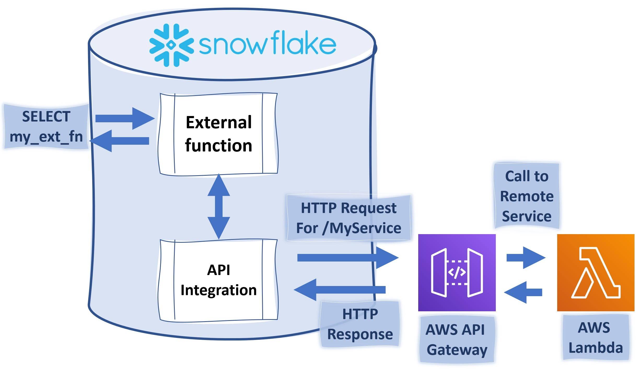
We will show you how to query and manipulate data across different solutions using the same SQL programming language.

The Solita Developer survey has become a tradition here at Solita and please check out the latest survey. It’s easy to see how SQL is dominating in a pool of many cool programming languages. It might take an average learner about two to three weeks to master the basic concepts of SQL and this is exactly what we will do with you.

Data modeling and real-time data

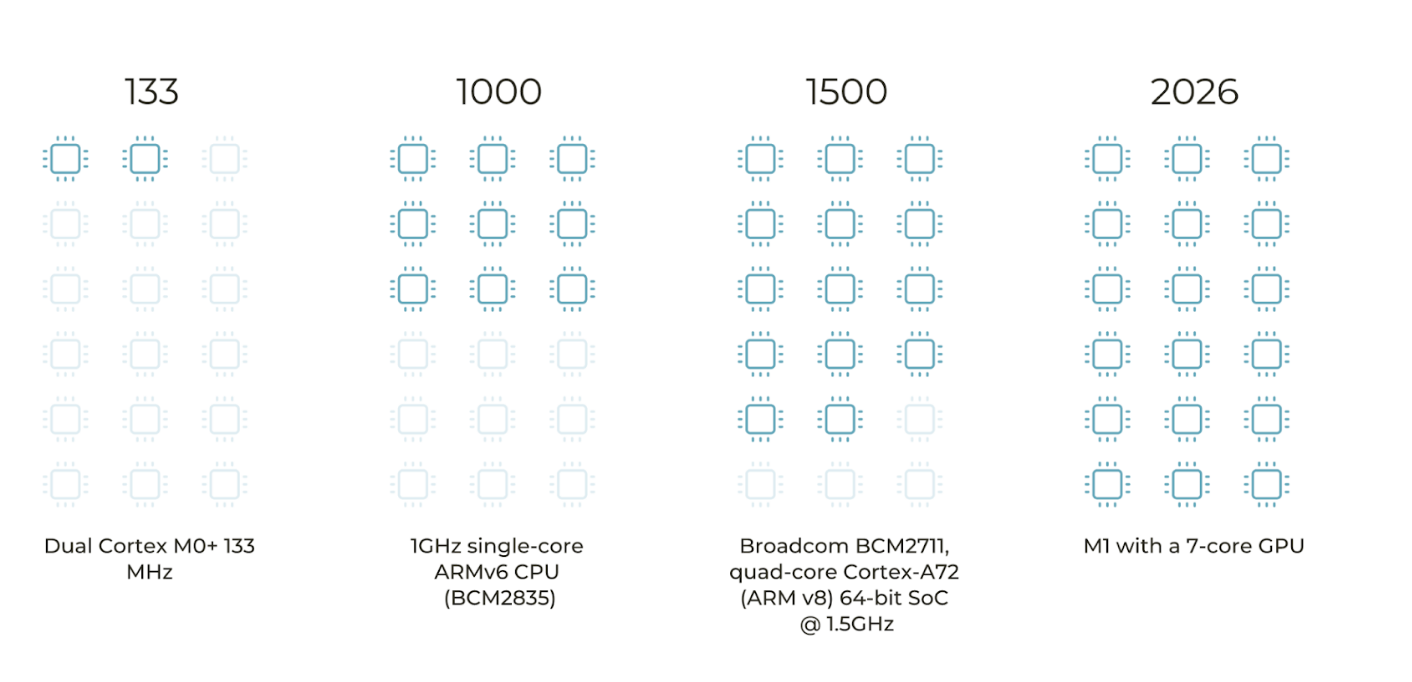
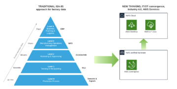
Operative technology (OT) solution have been real time from day one despite it’s also a question of illusion of real-time when it comes to IT systems. We could say that having network latency 5-15 ms towards Cloud and data processing with single-digit millisecond latency irrespective of the scale is considered near real time. This is important for Santa Claus and Industry 4.0 where autonomous fleet, robots and real-time processing in automation and control is a must have. Imagine situation where Santa’s autonomous sleigh with smart safety systems boosted computer vision (CV) able bypass airplanes and make smart decisions would have time of unit seconds or minutes – that would be a nightmare.

A data model is an abstract model that organizes elements of data and standardizes how they relate to one another and to the properties of real-world entities.

It’s easy to identify at least conceptual, logical and physical data models, where from the last one we are interested the most in this exercise to store and query data.

Back to the Future

Dimensional model heavily development by Ralph Kimball was breakthrough 1996 and had concepts like fact tables, dimension and ultimately creating a star schema. Challenge of this modeling is to keep conformed dimensions across the data warehouse and data processing can create unnecessary complexity.

One of the main driving factors behind using Data Vault is for both audit and historical tracking purposes. This methodology was developed by Daniel (Dan) Linstedt in early 2000. It has gain a lot of attraction being able to support especially modern cloud platform with massive parallel processing (MPP) of data loading and not to worry so much of which entity should be loaded first. Possibility even create data warehouse from scratch and just loading data in is pretty powerful when designing an idempotent system. 

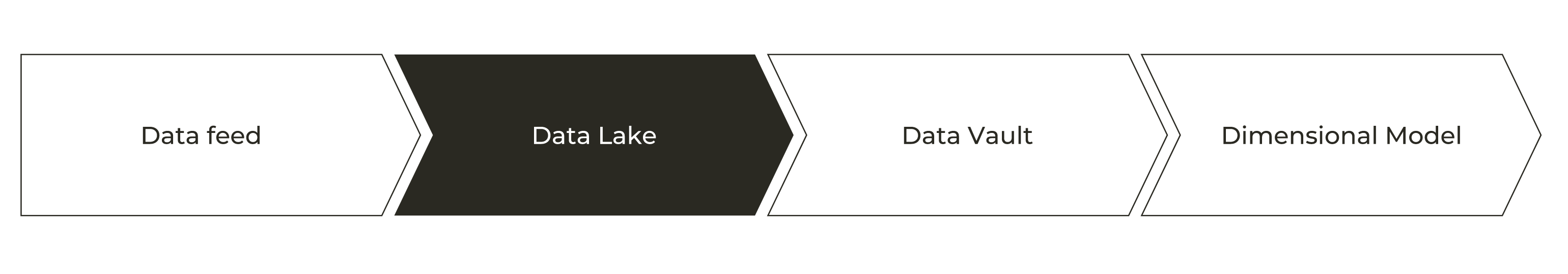
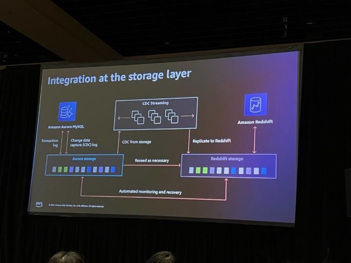
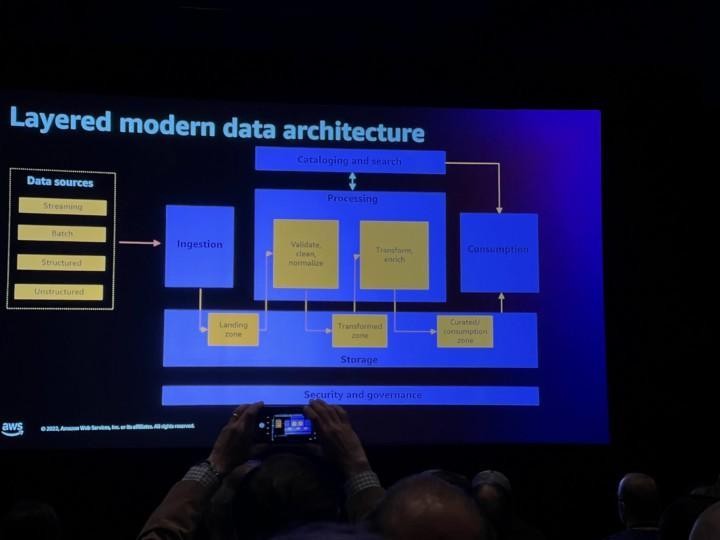
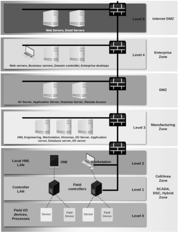
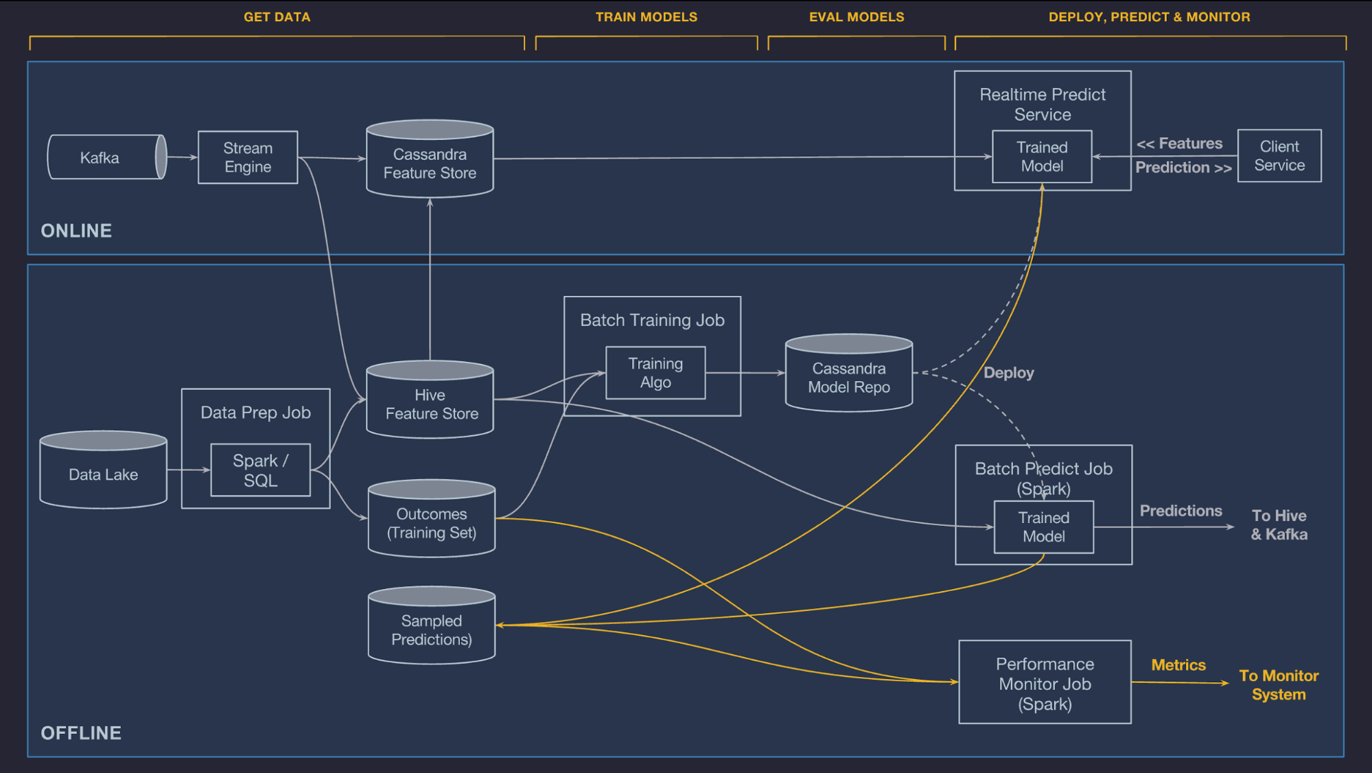
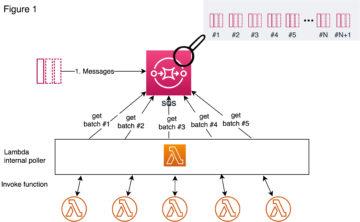
Quite typical data flow looks like picture above and like you already noticed this will have impact on how fast data is landed into applications and users. Theses for Successful Modern Data Warehousing are useful to read when you have time.

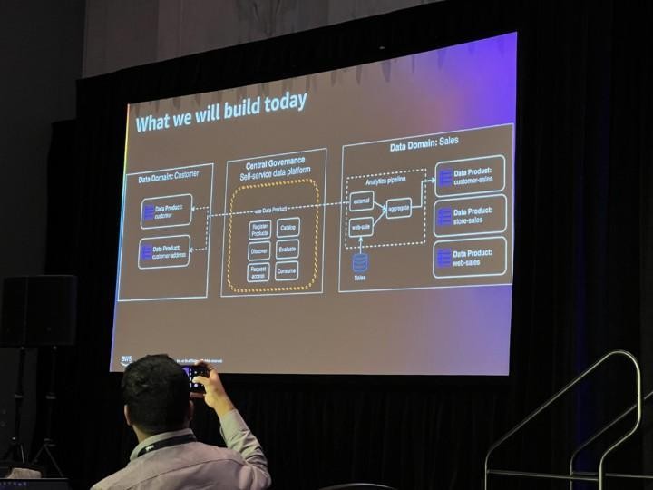
Data Mesh ultimate promise is to eliminate the friction to deliver quality data for producers and enable consumers to discover, understand and use the data at rapid speed. You could imagine this as data products in own sandboxes with some common control plane and governance. In any case to be successful you need expertise from different areas such as business, domain and data. End of the day Data Mesh does not take a strong position on data modeling.

Wide Tables / One Big Table (OBT) that is basically nested and denormalized tables is one modeling that is perhaps the mostly controversy. Shuffling data between compute instances when executing joins will have negative impact on performance (yes, you can e.g. replicate dimensional data to nodes and keep fact table distributed which will improve performance) and very often operational data structures produced by micro-services and exchanged over API are closer to this “nested” structure. Having same structure and logic for batch SQL as streaming SQL will ease your work.

Breaking down the OT data items to multiple different sub optimal data strictures inside IT systems will loose the single, atomic data entity. Having said this it’s possible to ingest e.g. Avro files to MPP, keeping the structure same as original file as and using evolving schemas to discovery new attributes. That can be then use as baseline to load target layers such as Data Vault.

One interesting concept called Activity Schema that is sold us as being designed to make data modeling and analysis substantially simpler, faster.

Contextualize data

For our industrial Santa Claus case one very important thing is how to create inventory and contextualize data. One very promising path is an augmented data catalog that will cover a bit later. For some reason there is material out there explaining how IoT data has no structure which is just incorrect. The only reason I can think is that kind of data asset was not fit to traditional data warehouse thinking.

Something to take a look is Apache Avro that is a language-neutral data serialization system, developed by Doug Cutting, the father of Hadoop. The other one is JSON is an open standard file format and data interchange format that uses human-readable text to store and transmit data objects consisting of attribute–value pairs and arrays. This is not solution for data modeling even more you will notice later on this blog post how those are very valuable on steaming data and having schema compared to other formats like CSV.

Business case for Santa

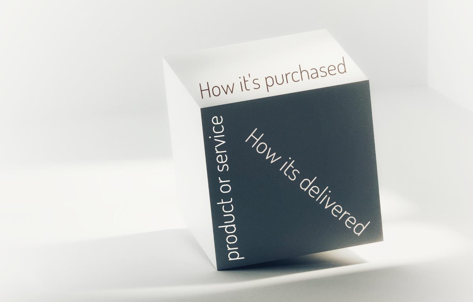
Like always everything starts with Why and solution discovery phase, what we actual want to build and would that have a business value. At Christmas time our business is around gifts and how to deliver those on time. Our model is a bit more simplified and will include operational technology systems such as assets (Santa’s workshop) and fleet (sleighs) operations. There might always be something broken so few maintenance needs are pushed to technicians (elfs). Distributed data platform is used for supply chain and logistics analytics to remove bottlenecks so business owners can be satisfied (Santa Claus and the team) and all gifts will be delivered to the right address just in time.

Case Santa’s workshop

We can later use OEE to calculate that workshop performance in order to produce high quality nice gifts. Data is ingested real time and contextualized so once a while Santa and the team will check how we are doing. In this specific case we know that using Athena we can find relevant production line data just querying the S3 bucket where all raw data is stored already.

Day 1 – creating a Santa’s table for time series data

Let’s create a very basic table to capture all data from Santa’s factory floor. You will notice there are different data types like bigint and string. You can even add comments to help others to later find what kind of data field should include. In this case raw data is Avro but you do not have to worry about that so let’s go.

CREATE EXTERNAL TABLE `raw`(

`seriesid` string COMMENT 'from deserializer',

`timeinseconds` bigint COMMENT 'from deserializer',

`offsetinnanos` bigint COMMENT 'from deserializer',

`quality` string COMMENT 'from deserializer',

`doublevalue` double COMMENT 'from deserializer',

`stringvalue` string COMMENT 'from deserializer',

`integervalue` int COMMENT 'from deserializer',

`booleanvalue` boolean COMMENT 'from deserializer',

`jsonvalue` string COMMENT 'from deserializer',

`recordversion` bigint COMMENT 'from deserializer'

) PARTITIONED BY (

`startyear` string, `startmonth` string,

`startday` string, `seriesbucket` string

)

Day 2 – query Santas’s data

Now we have a table and how to query that one ? That is easy with SELECT and taking all fields using asterix. It’s even possible to limit that to 10 rows which is always a good practice.

SELECT * FROM "sitewise_out"."raw" limit 10;

Day 3 – Creating a view from query

View is a virtual presentation of data that will help to organize assets more efficiently. One golden rule is still now to create many views on top of other views and keep the solution simple. You will notice that CREATE VIEW works nicely and now we have timeinseconds and actual factory floor value (doublevalue) captured. You can even drop the view using DROP command.

CREATE OR REPLACE VIEW "v_santa_data"

AS SELECT timeinseconds, doublevalue FROM "sitewise_out"."raw" limit 10;

Day 4 – Using functions to format dates to Santa

You noticed that timeinseconds is in Epoch so let’s use functions to have more human readable output. So we add a small from_unixtime function and combine that with date_format to have formatted output like we want. Perfect, now we know from which data Santa Claus manufacturing data originated.

SELECT date_format(from_unixtime(timeinseconds),'%Y-%m-%dT%H:%i:%sZ') , doublevalue FROM "sitewise_out"."raw" limit 10;

 Day 5 – CTAS creating a table

Using CTAS (CREATE TABLE AS SELECT) you can even create a new physical table easily. You will notice that Athena specific format has been added that you do not need on relational databases.

CREATE TABLE IF NOT EXISTS new_table_name

WITH (format='Avro') AS

SELECT timeinseconds , doublevalue FROM "sitewise_out"."raw" limit 10;

Day 6 – Limit the result sets

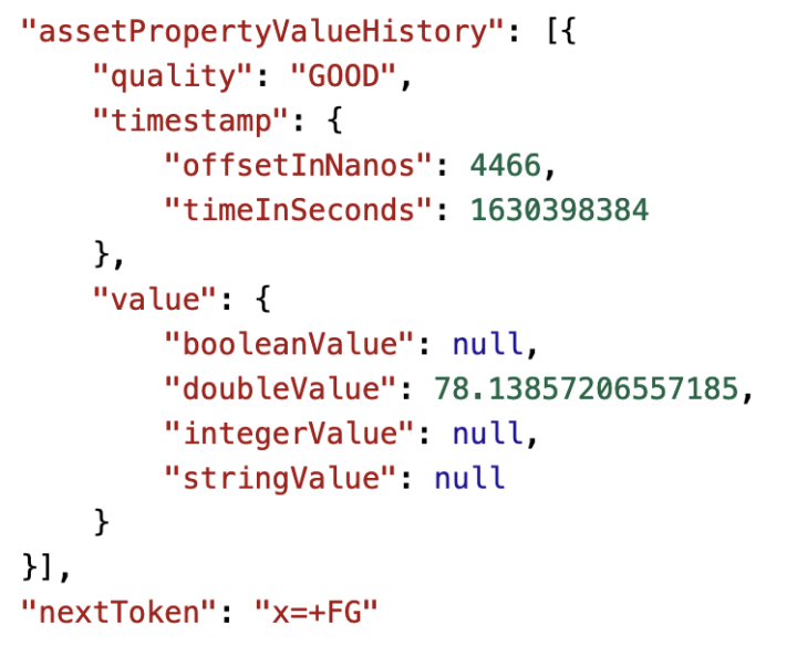
Now I want to limit the results to only those where the quality is Good.Adding a WHERE clause I can have only those rows printed to my output – that is cool!

SELECT * FROM "sitewise_out"."raw"  where quality='GOOD' limit 10;


Case Santa’s fleet

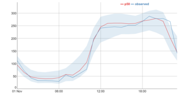
Now we jump into Santa’s fleet meaning sleights and there is few attribute we are interested like SleightD , IsSmartLock, LastGPSTime , SleightStateIDLatitude and Longitude. This data is time series that is ingested into our platform near real-time. Let’s use AWS Timestream service which is fast, scalable, and serverless time series database service for IoT and operational applications. A time series is a data set that tracks a sample over time. 

Day 7 – creating a table for fleet

You will notice very quickly that data model looks different than on relational database cases. There is no need beforehand to define table structure just executing CreateTable is enough.


Day 8- query the latest record

You can override time field using e.g. LastGPSTime, in this example we use time when data was ingested in, so getting the last movement of sleigh would be like this.

SELECT * FROM movementdb.tbl_movement
ORDER BY time DESC
LIMIT 1

Day 9- let’s check the last 24 hours movement

We can use time to filter our results and ordering on descending same time.

SELECT *
FROM "movementdb"."tbl_movement" 
WHERE time > ago(24h) 
ORDER BY time DESC

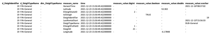
Day 10- latitude and longitude

We can find out latitude and longitude information easily and please note we are using IN operator to bet both to query result.

SELECT measure_name,measure_value::double,time 
FROM "movementdb"."tbl_movement" 
WHERE time > ago(24h) 
and measure_name in ('Longitude','Latitude')
ORDER BY time DESC LIMIT 10

Day 11- last connectivity info

Now we use 2 things so we group data based on sleigh id and find the maximum value. This will tell when sleigh was connected and sending data to our platform. There are plenty of functions to choose from so please check documentation.

SELECT greatest (time) as last_time, sleighId
FROM "movementdb"."tbl_movement" 
WHERE time > ago(24h) 
and measure_name = ('LastGPSTime')
group by sleighId,greatest (time)

Day 12- using conditions for smart lock data

CASE is very powerful to manipulate the query results so in this example we use that do indicate better if sleigh had smart lock.

SELECT time, measure_name,
CASE 
WHEN measure_value::boolean = true THEN 'Yes we have a smart lock'
ELSE 'No we do not that kind of fancy locks'
END AS smart_lock_info
FROM "movementdb"."tbl_movement"
WHERE time between ago(1d) and now() 
and measure_name='IsSmartLock'

Day 13- finding the latest battery level on each fleet equipment

This would be a bit more complex so we have one query to find max value of battery level and then we later join that to base data so on each record we know the latest battery level in the past 24 hours. Please notice we are using INNER join in this example.

WITH latest_battery_time as (
select 
d_sleighIdentifier, 
max(time) as latest_time 
FROM 
"movementdb"."tbl_movement" 
WHERE 
time between ago(1d) 
and now() 
and measure_name = 'Battery' 
group by 
d_sleighIdentifier
) 
SELECT 
b.d_sleighIdentifier, 
b.measure_value :: double as last_battery_level 
FROM 
latest_battery_time a 
inner join "movementdb"."tbl_movement" b on a.d_sleighIdentifier = b.d_sleighIdentifier 
and b.time = a.latest_time 
WHERE 
b.time between ago(1d) 
and now() 
and b.measure_name = 'Battery'

Day 14- distinct values

The SELECT DISTINCT statement is used to return only distinct (different) values. This is so create and also very misused when removing duplicates etc. when actual problem can be on JOIN conditions.

SELECT 
DISTINCT (d_sleighIdentifier) 
FROM 
"movementdb"."tbl_movement"

Day 15- partition by is almost magic

The PARTITION BY clause is a subclause of the OVER clause. The PARTITION BY clause divides a query’s result set into partitions. The window function is operated on each partition separately and recalculate for each partition. This is almost a magic and that can be used in several ways like in this example identify last sleigh Id.

select 
d_sleighIdentifier, 
SUM(1) as total, 
from 
(
SELECT 
*, 
first_value(d_sleighIdentifier) over (
partition by d_sleighTypeName 
order by 
time desc
) lastaction 
FROM 
"movementdb"."tbl_movement" 
WHERE 
time between ago(1d) 
and now()
) 
GROUP BY 
d_sleighIdentifier, 
lastaction

Day 16- interpolation (values of missing data points)

Timestream and few other IoT services supports linear interpolation, enabling to estimate and retrieve the values of missing data points in their time series data. This will come very handy when our fleet is not connected all the time, in this example we used it for our smart sleight battery level.

WITH rawseries as (
select 
measure_value :: bigint as value, 
time as d_time 
from 
"movementdb"."tbl_movement" 
where 
measure_name = 'Battery'
), 
interpolate as (
SELECT 
INTERPOLATE_LINEAR(
CREATE_TIME_SERIES(d_time, value), 
SEQUENCE(
min(d_time), 
max(d_time), 
1s
)
) AS linear_ts 
FROM 
rawseries
) 
SELECT 
time, 
value 
FROM 
interpolate CROSS 
JOIN UNNEST(linear_ts)

Case Santa’s  master data

Now we jump into Master Data when factory and fleet is up are covered. In this very complex supply chain system customer data is very typical transactional data and in this exercise we keep it very atomic having stored only very basic info into DynamoDB that is a fully managed, serverless, key-value NoSQL database designed to run high-performance applications at any scale. We use this data to on IoT data streams for join, filtering and other purposes in fast manner. Good to remember that DynamoDB is not build for complex query patterns so it’s best on it’s original key=value data query pattern.

Day 17- adding master data

We upload our customer data into DynamoDB so called “items” based om the list received from Santa.

{
"customer_id": {
"S": "AJUUUUIIIOS"
},
"category_list": {
"L": [
{
"S": "Local Businesses"
},
{
"S": "Restaurants"
}
]
},
"homepage_url": {
"S": "it would be here"
},
"founded_year": {
"N": "2021"
},
"contract": {
"S": "NOPE"
},
"country_code": {
"S": "FI"
},
"name": {
"S": ""
},
"market_stringset": {
"SS": [
"Health",
"Wellness"
]
}
}

Day 18- query one customer item

Amazon DynamoDB supports PartiQL, a SQL-compatible query language, to select, insert, update, and delete data in Amazon DynamoDB. That is something we will use too speed up things. Let’s first query one customer data asset.

SELECT * FROM "tbl_customer" where customer_id='AJUUUUIIIOS'

Day 18- update kids information

Using the same PartiQL you can update item to have new attributes with one go.

UPDATE "tbl_customer" 
SET kids='2 kids and one dog' 
where customer_id='AJUUUUIIIOS'

Day 19- contains function

Now we can easily check that form marketing data who was interested on Health using CONTAINS. Many moderns database engines have native support for semi-structured data, including: Flexible-schema data types for loading semi-structured data without transformation. If you are not already familiar please take a look on AWS Redshift and Snowflake.

SELECT * FROM "tbl_customer" where contains("market_stringset", 'Health')

Day 20- inserting a new customer

Using familiar SQL like it’s very straightforward to add one new item.

INSERT INTO "tbl_customer" value {'name' : 'name here','customer_id' : 'A784738H'}

Day 21- missing data

Using a special MISSING you can find those where some attribute is not present easily.

SELECT * FROM "tbl_customer" WHERE "kids" is MISSING

Day 22- export data into s3

With one command you can export data from DynamoDB to S3 so let’s do that one based on documentation. AWS and others do have support for something called Federated Query where you can run SQL queries across data stored in relational, non-relational, object, and custom data sources. This federated feature we will cover later with You.

Day 23- using S3 select feature

Now you have data stored to  S3 bucket and there is holder called /data so you can even use SQL to query S3 stored data. This will find relevant information for customer_id.

Select s.Item.customer_id from S3Object s

Day 24- s3 select to find right customer

You can even use customer Id to restrict data returned to you.

Select s.Item.customer_id from S3Object s where s.Item.customer_id.S ='AJUUUUIIIOS'


That’s all, I hope you get some glimpse how useful SQL is even you have different services and you might first think this will never be possible to use same kind of language of choice. Please do remember when some day You might be building next generation artificial intelligence and analysis platform with us knowing few data modeling techniques and SQL is a very good start.

You might be interested Industrial equipment data at scale for factory floor or manage your fleet at scale so let’s keep fresh mind and have a very nice week !


vision

The Industrial Revolution 6.0

Strength of will, determination, perseverance, and acting rationally in the face of adversity

The Industrial Revolution

The European Commission has taken a very active role to define Industry 5.0 and it complements Industry 4.0 for transformation of sustainable, human-centric and resilient European industry.

Industry 5.0 provides a vision of industry that aims beyond efficiency and productivity as the sole goals, and reinforces the role and the contribution of industry to society. https://ec.europa.eu/info/research-and-innovation/research-area/industrial-research-and-innovation/industry-50_en

Finnish industry is affected by the pandemic, the fragmentation global supply chains and dependency of suppliers all around the world. Finnish have something called “sisu”. It’s a Finnish term that can be roughly translated into English as strength of will, determination, perseverance, and acting rationally in the face of adversity. That might be one reason why in Finland group of people are already defining Industry 6.0 and also one of the reasons we wanted to share our ideas using blog posts such as:

  1. Smart and Connected Factories
  2. Factory Floor and Edge computing
  3. Industrial data contextualization at scale
  4. AWS SageMaker Pipelines – Making MLOps easier for the Data Scientist
  5. Productivity and industrial user experience
  6. Cloud data transformation
  7. Illusion of real-time
  8. Manufacturing security hardening

It’s not well defined where the boundaries on each industrial revolution really are. We can argue that first Industry 1.0 was around 1760 when transition to new manufacturing processes using water and steam was happening.  Roughly 1840 the second industrial revolution was referred to as “The Technological Revolution” where one component was superior electrical technology which allowed for even greater production. Industry 3.0 introduced more automated systems onto the assembly line to perform human tasks, i.e. using Programmable Logic Controllers (PLC).

Present 

The Fourth Industrial Revolution (Industry 4.0) will incorporate storage systems and production facilities that can autonomously exchange information. How to deliverer and purchase any service or product will have on these 3 dimensions two categories: physical and digital.

IoT has a bit of inflation as a word and the few biggest hype cycles are past life- which is a good thing. The Internet of things (IoT) plays very important role to enable smart connected devices and extend the possibility to Cloud computing. Companies are already creating cyber-physical systems where machine learning (ML) is built into product-centered thinking. Few of the companies have a digital twin that serves as the real-time digital counterpart of a physical object or process.

In Finland with a long history of factory, process and manufacturing companies this is reality and bigger companies are targeting for faster time to market, quality and efficiency. Rigid SAP processes combined with yearly budgets are not blocking future looking products and services – we are past that time. There are great initiatives for sensor networks and edge computing for environment analysis. Software enabled intelligent products, new better offerings based on real usage and how to differentiate on market is everyday business to many of us in the industrial domain.

Future

“When something is important enough, you do it even if the odds are not in your favor.” Elon Musk

World events have pushed industry to rethink how to build and grow business in a sustainable manner. Industry 5.0 is being said to be the revolution in which man and machine reconcile and find ways to work together to improve the means and efficiency of production.  Being on stage or watching your fellow colleagues you can hear words like human-machine co-creative resilience, mass-customization,  sustainability and circular economy. Product complexity is increasing at the same time with ever-increasing customer expectations.

Industry 6.0 exists only in whitepapers but that does not mean that “customer driven virtualized antifragile manufacturing” could be real some day. Hyperconnected factories and dynamic supply chains would most probably benefit all of us. Some are referring to industrial change same way as hyperscalers such as AWS are doing for selling cloud capacity. There are challenges for sure like “Lot Size One” to be economically feasible. One thing is for sure that all models and things will merge, blur and convergence.


Building the builders

“My biggest mistake is probably weighing too much on someone’s talent and not someone’s personality. I think it matters whether someone has a good heart.” – Elon Musk

One fact is that industrial life is not super interesting for millennials. It looks old fashioned so to have a future professional is a must have. Factory floor might not be as interesting as it was a few decades ago. Technology possibilities and cloud computing will boost to have more different people to have interest towards industrial solutions. A lot of ecosystems exist with little collaboration and we think it’s time to change that by reinventing business models, solutions and onboarding more fresh minded people for industrial solutions.

That is one reason we have packaged kickstarts to our customers and anyone interested can grow with us.


Manufacturing security hardening

Securing IT/OT integration


Last time my colleague Ripa and I discussed about industrial UX and productivity. This time I focus on factory security especially in situations when factories will be connected to the cloud.

Historical habits 

As we know for a long time manufacturing OT workloads were separated from IT workloads. Digitalization, IoT and edge computing enabled IT/OT convergence and made it possible to take advantage of cloud services.

Security model at manufacturing factories has been based on isolation where the OT workload could be isolated and even fully air-gapped from the company’s other private clouds. I recommend you to take a look at the Purdue model back from the 1990s, which was and still is the basis for many factories for giving guidance for industrial communications and integration points. It was so popular and accepted that it became the basis for the ISA-95 standard (the triangle I drew in a blog post). 

Now with new possibilities with the adoption of cloud, IoT, digitalization and enhanced security we need to think: 

Is the Purdue model still valid and is it just slowing down moving towards smart and connected factories?

Purdue model presentation aligned to industrial control system


Especially now that edge computing (manufacturing cloud) is becoming more sensible, we can process the data already at level 1 and send the data to the cloud using existing secured network topology. 

Is the Purdue model slow down new thinking ? Should we have Industrial Edge computing platform that can connect to all layers?


Well architected

Thinking about the technology stack from factory floor up to AWS cloud data warehouses or visualizations, it is huge! It’s not so straightforward to take into account all the possible security principles to all levels of your stack. It might even be that the whole stack is developed during the last 20 years, so there will be legacy systems and technology dept, which will slow down applying modern security principles. 

In the following I summarize 4 main security principles you can use in hybrid manufacturing environments:

  • Is data secured in transit and at rest ? 

Use encryption and if possible enforce it. Use key and certificate management with scheduled rotation. Enforce access control to data, including backups and versions as well. For hardware, use Trusted Platform Module (TPM) to store keys and certificates.

  • Are all the communications secured ? 

Use TLS or IPsec to authenticate all network communication. Implement network segmentation to make networks smaller and tighten trust boundaries. Use industrial protocols like OPC-UA.

  • Is security taken in use in all layers ? 

Go through all layers of your stack and verify that you cover all layers with proper security control.

  • Do we have traceability ? 

Collect log and metric data from hardware and software, network, access requests and implement monitoring, alerting, and auditing for actions and changes to the environment in real time.


Secured data flow 

Following picture is a very simplified version of the Purdue model aligned to manufacturing control hierarchy and adopting AWS cloud services. It focuses on how manufacturing machinery data can connect to the cloud securely. Most important thing to note from the picture is that network traffic from on-prem to cloud is private and encrypted. There is no reason to route this traffic through the public internet. 

Purdue model aligned to manufacturing control hierarchy adopting AWS cloud


You can establish a secure connection between the factory and AWS cloud by using AWS Direct Connect or AWS Site-to-Site VPN. In addition to this I recommend using VPC endpoints so you can connect to AWS services without a public IP address. Many AWS services support VPC endpoints, including AWS Sitewise and IoT Core.

Manufacturing machinery is on layers 0-2. Depending on the equipment trust levels it’s a good principle to divide the whole machinery into cells / sub networks to tighten trust boundaries. Machinery with different trust levels can be categorized in its own cells. Using industrial protocols, like OPC-UA, brings authentication and encryption capabilities near the machinery. I’m very excited about the possibility to do server initiated connections (reverse connect) on OPC-UA, which makes it possible for clients to communicate with server without firewall inbound port opening.

As you can see from the picture, data is routed through all layers of and looks like layers IDMZ (Industrial Demilitarized Zone), 4 and 5 are almost empty. As discussed earlier, only for connecting machinery to the cloud via secure tunneling we could bypass some layers. But for other use cases the layers are still needed. If for some reason we need to route factory network traffic to AWS Cloud through the public internet, we need a TLS proxy on IDMZ to encrypt the traffic and protect the factory from DDoS attacks (Distributed Denial of Service attack).

The edge computing unit on Layer 3 is a AWS Greengrass device which ingests data from factory machinery, processes the data with ML and sends only the necessary data to the cloud. The unit can also discuss and ingest data from Supervisory Control and Data Acquisition (SCADA), and Distributed Control System (DCS) and other systems from manufacturing factories. AWS Greengrass uses x509 certificate based authentication to AWS cloud. Idea is that the private key will not leave from the device and is protected and stored in the device’s TPM module. All the certificates are stored to AWS IoT Core and can be integrated to custom PKI. For storing your custom CA’s (Certificate Authority) you can use AWS ACM. I strongly recommend to design and build certificate lifecycle policies and enforce certificate rotation for reaching a good security level.

One great way of auditing your cloud IoT security configuration is to audit it with AWS IoT Device Defender. Also you can analyse the factory traffic real-time, find anomalies and trigger security incidents automatically when needed.


Stay tuned

Security is our best friend, you don’t need to be afraid of it.

Build it to all layers, from bottom to top in as early a phase as possible. AWS has the security capabilities to connect private networks to the cloud and do edge computing and data ingesting in a secure way. 

Stay tuned for next posts and check out our Connected Factory Kickstart if you haven’t yet

https://www.solita.fi/en/solita-connected/


Illusion of real-time

Magic is the only honest profession. A magician promises to deceive you and he does.

Cloud data transformation

Tipi shared thoughts on how data assets could be utilized on Cloud. We had few question after blog post and one of those was “how to tackle real time requirements ?

Let’s go real time ?

Real-time business intelligence is a concept describing the process of delivering business intelligence or information about business operations as they occur. Real time means near to zero latency and access to information whenever it is required.

We all remember those nightly batch loads and preprocessing data –  waiting a few hours before data is ready for reports. Someone is looking if sales numbers are dropped and the manager will ask quality reports from production. Report is evidence to some other team what is happening in our business.

Let’s go back to the definition that says “information whenever it is required” so actually for some of the team(s) even one week or day can be realtime. Business processes and humans are not software robots so taking action based on any data will take more than a few milliseconds so where is this real time requirement coming from ?

Marko had a nice article related to OT systems and Factory Floor and Edge computing. Any factory issue can be a major pain and downtime is not an option and explained how most of the data assets like metrics and logs must be available immediately in order to recover and understand the root cause.

Hyperscalers and real time computing

In March 2005, Google acquired the web statistics analysis program Urchin, later known as Google Analytics. That was one of the customer facing solutions to gather massive amount of data. Industrial protocols like Modbus from 1970 was designed to work real time on that time and era. Generally speaking real time computing has three categories:

  • Hard – missing a deadline is a total system failure.
  • Firm – infrequent deadline misses are tolerable, but may degrade the system’s quality of service. The usefulness of a result is zero after its deadline.
  • Soft – the usefulness of a result degrades after its deadline, thereby degrading the system’s quality of service.

So it’s easy to understand that airplane turbine and rolling 12 months sales forecast have different requirements. .

What is the cost of (data) delay ?

“A small boat that sails the river is better than a large ship that sinks in the sea.”― Matshona Dhliwayo

We can simply estimate the value a specific feature would bring in after its launch and multiply this value with the time it will take to build. That will tell the economic impact that postponing a task will have.

High performing teams can do cost of delay estimation to understand which task should take first.  Can we calculate and understand the cost of delayed data? How much that will cost to your organization if service or product must be postponed because you are missing data or you can not use it.

Start defining real-time

You can easily start discussing what kind of data is needed to improve customer experience.  Real time requirements might be different for each use case and that is totally fine. It’s a good practice to specify near real time requirements in factual numbers and few examples. It’s good to remember that end to end can have totally different meanings. Working with OT systems for example the term First Mile is used when protect and connect OT systems with IT.

Any equipment failure must be visible to technicians at site in less than 60 seconds. ― Customer requirement

Understand team topologies

Incorrect team topology can block any near real time use cases. That means that adding each component and team deliverable to work together might end up having unexpected data delays. Or in the worst case scenario a team is built too much around one product / feature that will have come a bottleneck later when building more new services.

Data as a product refers to an idea where the job of the data team is to provide the data that the company needs. Data as a Service team partners with stakeholders and have more functional experience and are responsible for providing insight as opposed to rows and columns. Data Mesh is about the logical and physical interconnections of the data from producers through to consumers.

Team topologies will have a huge impact on how data driven services are built and can data land to business case purposes just on the right time.

Enable Edge streaming and APIs capabilities

On cloud services like AWS Kinesis is great, it is a scalable and durable real-time data streaming service that can continuously capture gigabytes of data per second. Apache Kafka is a framework implementation of a software bus using stream-processing. Apache Spark is an open-source unified analytics engine for large-scale data processing.

I am sure that at least one of these you are already familiar with. In order to control data flow we have two parameters: amount of messages and time. Which will come first will se served.

 Is your data solution idempotent and able to handle data delays ? ― Customer requirement

Modern purpose-built databases have capability to process streaming data. Any extra layer of data modeling will add a delay for data consumption. On Edge we typically run purpose-built robust database services in order to capture all factory floor events with industry standard data models.

Site and Cloud API is a contact between different parties and will improve connectivity and collaboration. API calls on Edge works nicely and you can have data available in less than 70-300ms from Cloud endpoint (example below). Same data is available on Edge endpoint where client response is even faster so building factory floor applications is easy.

curl --location --request GET 'https://data.iotsitewise.eu-west-1.amazonaws.com/properties/history?assetId=aa&maxResults=1&propertyId=pp --header 'X-Amz-Date: 20211118T152104Z' --header 'Authorization: AWS4-HMAC-SHA256 Credential=xxx, SignedHeaders=host;x-amz-date, Signature=xxxx

Quite many databases has built-in Data API. It’s still good to remember that underlying engine, data model and many factors will determine how scalable solution really is.

AWS GreenGrass StreamManager is a component that enables you to process data streams to transfer to the AWS Cloud from Greengrass core devices. Other services like Firehose is supported using specific aws.greengrass.KinesisFirehose component. These components will support also building Machine Learning (ML) features on Edge as well.


Conclusion

Business case will define the requirement of real time. Build your near real time capabilities according to your future proof architecture – adding real time capabilities later might come almost impossible. 

If business case is not clear enough what should I do ? Maybe a cup of tea, relax and read blog post from Johannes The gap between design thinking and business impact

You might be interested our kickstarts Accelerate cloud data transformation ​and Industrial equipment data at scale

Let’s stay fresh-minded !


Accelerate cloud data transformation

Cloud data transformation

Data silos and unpredicted costs preventing innovation

Cloud database race ?

One of the first cloud services was S3 launched in 2006.  AWS Hadoop based Amazon SimpleDB  was released in 2007 and after that there have been many nice cloud database products from multiple cloud hyperscalers. Database as a service (DBaaS) has been a prominent service when customers are looking for scaling, simplicity and taking advantage of the ecosystem. It has been estimated that the Cloud database and DBaaS market was estimated to be USD 12,540 Million by 2020, so no wonder there is a lot of activity. Looking from a customer point of view this is excellent news when the cloud database service race is on and new features are popping up and same time usage costs are getting lower. I can not remember the time when creating a global solution backed by a database would be so cost efficient as it is now.


Why should I move data assets to the Cloud ?

There are few obvious reasons like rapid setup, cost efficiency, scaling solutions and integration to other Cloud services. That will give nice security enforcement in many cases where old school username and password is not used like in some on premises systems still do.


“No need to maintain private data centers”, “No need to guess capacity”


Cloud computing instead typical on premises setup is distributed by nature, so computing and storage are separated. Data replication to other regions is supported out of the box in many solutions, so data can be stored as close as possible to end users for best in class user experience.

In the last few years even more database service can work seamlessly with on premises and cloud. Almost all data related cases have aspects of machine learning nowadays and Cloud empowers teams to enable machine learning in several different ways: in built into database services, purpose-built services or using native integrations. Just using the same development environment and using industry standard SQL you can do all ML phases easily. Database integrated AutoML aims to empower developers to create sophisticated ML models without having to deal with all the phases of ML – that is a great opportunity for any Citizen data scientist !


Purpose build databases to support diverse data models

Beauty of cloud comes rapidly with flexibility and pay as you go model with very real time cost monitoring. You can cherry pick the best purpose-built database (relational, key-value, document, in-memory, graph, time series, wide column, and ledger databases.) to suit your use case, data models and avoid building one big monolithic solution.

Snowflake is one of the few enterprise-ready cloud data warehouses that brings simplicity without sacrificing features and can be operated on any major cloud platform. Amazon Relational Database Service (Amazon RDS) makes it easy to set up, operate, and scale to any relational database in the cloud. Amazon Timestream is a nice option for serverless, super fast time series processing and near real time solutions. You might have a Hadoop system or running a non-scalable relational database on premises and think about how to get started on a journey for improved customer experience and digital services?

Success for your cloud data migration

We have worked with our customers to build a Data Migration strategy. That will help in understanding the migration options, create a plan and also validate future proof architecture.

Today we share with you here a few tips that might help you when planning data migrations.

  1. Employee experience – embrace your team, new possibilities and replace pure technical approach to include commitment from your team developers. Domain knowledge of data assets and applications is very important and building a trust to new solutions from day one.
  2. Challenge your partner of choice. There is more than lift and shift or creating all from scratch options. It might be that all data assets are not needed or useful anymore. Our team is working on a vertical slicing approach where the elephant is splitted to manageable pieces. Using state of the art accelerator solutions we can make an inventory using real life metrics. Let’s make sure that you can avoid the big bang and current systems can operate without impact even when building new systems.
  3. Bad design and technical debt of legacy systems. It’s very typical that old systems’ performance and design can be broken already.  That is something which is not visible to all stakeholders and when doing the first Cloud transformation all that will come visible will pop up. Prepare yourself for surprises – take that as an opportunity to build more robust architecture. Do not try to fix all problems at once !
  4. Automation to the bones. In order to be able to try and replay data make sure everything is fully automated including database, data loading and integrations. So, making a change is fun and not something to be careful of. It’s very hard to build DataOps to on premises systems because of the nature of operating models, contracts and hardware limitations. In Cloud those are not the blockers anymore.
  5. Define workloads and scope ( no low hanging fruits only) . Taking one database and moving that to the Cloud can not be used as any baseline when you have hundreds of databases. Metrics from the first one should not be used as a matrix multiplied by the amount of databases when thinking about the whole project scope. Take a variety of different workloads and solutions, some even the hard one to first sprint. It’s better to start immediately and not wait for any target systems because on Cloud that is totally redundant.
  6. Welcome Ops model improvement. On Cloud database metrics of performance (and any other kind) and audit trails are all visible so creating a more proactive and risk free ops model is at your fingertips. My advice is not to copy the existing Ops model with the current SLA as it is. High availability and recovery are different things – so do not mix those.
  7. Going for meta driven DW. In some cases choosing state of the art automated warehouse like Solita Agile Data Engine (ADE) will boost your business goals when you are ready to take a next step.


Let’s kick the Cloud Data transformation ongoing !

Take advantage of cloud when building digital services with less money and faster with our Accelerate cloud data transformation kickstart

You might be interested also Migrating to the cloud isn’t difficult, but how to do it right?

Productivity and industrial user experience

Digital employee is not software robot


The last post was about data contextualisation and today on this video blog post we talk about the Importance of User Experience in an Industrial Environment.

UX versus employee experience

User Experience (UX) design is the process design teams use to create products that provide meaningful and relevant experiences to users. 

Employee experience is a worker’s perceptions about his or her journey through all the touchpoints at a particular company, starting with job candidacy through to the exit from the company. 

Using modern, digital tools and platforms can support employee experience and create competitive advantage. Especially working on factory systems and remote locations it’s important to keep good productivity and one option is cloud based manufacturing.

Stay tuned for more and check our Connected Factory kickstart:

https://www.solita.fi/en/solita-connected/

AWS SageMaker Pipelines – Making MLOps easier for the Data Scientist

SageMaker Pipelines is a machine learning pipeline creation SDK designed to make deploying machine learning models to production fast and easy. I recently got to use the service in an edge ML project and here are my thoughts about its pros and cons. (For more about the said project refer to Solita data blog series about IIoT and connected factories https://data.solita.fi/factory-floor-and-edge-computing/)

Example pipeline

Why do we need MLOps?

First, there were statistics then came the emperor’s new clothes – machine learning, a rebranding of old methods accompanied with new ones emerged. Fast forward to today and we’re all the time talking about this thing called “AI”, the hype is real, it’s palpable because of products like Siri and Amazon Alexa.

But from a Data Scientist point of view, what does it take to develop such a model? Or even a simpler model, say a binary classifier? The amount of work is quite large, and this is only the tip of the iceberg. How much more work is needed to put that model into the continuous development and delivery cycle?

For a Data Scientist, it can be hard to visualize what kind of systems you need to automate everything your model needs to perform its task. Data ETL, feature engineering, model training, inference, hyperparameter optimization, performance monitoring etc. Sounds like a lot to automate?

(Hidden technical debt in machine learning https://proceedings.neurips.cc/paper/2015/file/86df7dcfd896fcaf2674f757a2463eba-Paper.pdf)


This is where MLOps comes to the picture, bridging DevOps CI/CD practices to the data science world and bringing in some new aspects as well. You can see more information about MLOps from previous Solita content such as https://www.solita.fi/en/events/webinar-what-is-mlops-and-how-to-benefit-from-it/ 

Building an MLOps infrastructure is one thing but learning to use it fluently is also a task of its own. For a Data Scientist at the beginning of his/her career, it could seem too much to learn how to use cloud infrastructure as well as learn how to develop Python code that is “production” ready. A Jupyter notebook outputting predictions to a CSV file simply isn’t enough at this stage of the machine learning revolution.

(The “first” standard on MLOps, Uber Michelangelo Platform https://eng.uber.com/michelangelo-machine-learning-platform/)


A Jupyter notebook outputting predictions to a CSV file simply isn’t enough at this stage of the machine learning revolution.

Usually, companies that have a long track record of Data Science projects have a few DevOps, Data Engineer/Machine Learning Engineer roles working closely with their Data Scientists teams to distribute the different tasks of production machine learning deployment. Maybe they even have built the tooling and the infrastructure needed to deploy models into production more easily. But there are still quite a few Data Science teams and data-driven companies figuring out how to do this MLOps thing.

Why should you try SageMaker Pipelines?

AWS is the biggest cloud provider ATM so it has all the tooling imaginable that you’d need to build a system like this. They are also heavily invested in Data Science with their SageMaker product and new features are popping up constantly. The problem so far has been that there are perhaps too many different ways of building a system like this.

AWS tries to tackle some of the problems with the technical debt involving production machine learning with their SageMaker Pipelines product. I’ve recently been involved in project building and deploying an MLOps pipeline for edge devices using SageMaker Pipelines and I’ll try to provide some insight on why it is good and what is lacking compared to a completely custom-built MLOps pipeline.

The SageMaker Pipelines approach is an ambitious one. What if, Data Scientists, instead of having to learn to use this complex cloud infrastructure, you could deploy to production just by learning how to use a single Python SDK (https://github.com/aws/sagemaker-python-sdk)? You don’t even need the AWS cloud to get started, it also runs locally (to a point).

SageMaker Pipelines aims at making MLOps easy for Data Scientists. You can define your whole MLOps pipeline in f.ex. A Jupyter Notebook and automate the whole process. There are a lot of prebuilt containers for data engineering, model training and model monitoring that have been custom-built for AWS. If these are not enough you can use your containers enabling you to do anything that is not supported out of the box. There are also a couple of very niche features like out-of-network training where your model will be trained in an instance that has no access to the internet mitigating the risk of somebody from the outside trying to influence your model training with f.ex. Altered training data.

You can version your models via the model registry. If you have multiple different use cases for the same model architectures with differences being in the datasets used for training it’s easy to select the suitable version from SageMaker UI or the python SDK and refactor the pipeline to suit your needs.  With this approach, the aim is that each MLOps pipeline has a lot of components that are reusable in the next project. This enables faster development cycles and the time to production is reduced. 

SageMaker Pipelines logs every step of the workflow from training instance sizes to model hyperparameters automatically. You can seamlessly deploy your model to the SageMaker Endpoint (a separate service) and after deployment, you can also automatically monitor your model for concept drifts in the data or f.ex. latencies in your API. You can even deploy multiple versions of your models and do A/B testing to select which one is proving to be the best.

And if you want to deploy your model to the edge, be it a fleet of RaspberryPi4s or something else, SageMaker provides tooling for that also and it seamlessly integrates with Pipelines.

You can recompile your models for a specific device type using SageMaker Neo Compilation jobs (basically if you’re deploying to an ARM etc. device you need to do certain conversions for everything to work as it should) and deploy to your fleet using SageMaker fleet management.

Considerations before choosing SageMaker Pipelines

By combining all of these features to a single service usable through SDK and UI, Amazon has managed to automate a lot of the CI/CD work needed for deploying machine learning models into production at scale with agile project development methodologies. You can also leverage all of the other SageMaker products f.ex. Feature Store or Forekaster if you happen to need them. If you’re already invested in using AWS you should give this a try.

Be it a great product to get started with machine learning pipelines it isn’t without its flaws. It is quite capable for batch learning settings but there is no support as of yet for streaming/online learning tasks. 

And for the so-called Citizen Data Scientist, this is not the right product since you need to be somewhat fluent in Python. Citizen Data Scientists are better off with BI products like Tableau or Qlik (which use SageMaker Autopilot as their backend for ML) or perhaps with products like DataRobot. 

And in a time where software products are high availability and high usage the SageMaker EndPoints model API deployment scenario where you have to pre-decide the number of machines serving your model isn’t quite enough.

 In e-commerce applications, you could run into situations where your API is receiving so much traffic that it can’t handle all the requests because you didn’t select a big enough cluster to serve the model with. The only way to increase the cluster size in SageMaker Pipelines is to redeploy a new revision within a bigger cluster. It is pretty much a no brainer to use a Kubernetes cluster with horizontal scaling if you want to be able to serve your model as the traffic to the API keeps increasing.

Overall it is a very nicely packaged product with a lot of good features. The problem with MLOps in AWS has been that there are too many ways of doing the same thing and SageMaker Pipelines is an effort for trying to streamline and package all those different methodologies together for machine learning pipeline creation.

It’s a great fit if you work with batch learning models and want to create machine learning pipelines really fast. If you’re working with online learning or reinforcement models you’ll need a custom solution. And if you are adamant that you need autoscaling then you need to do the API deployments yourself, SageMaker endpoints aren’t quite there yet. For references to a “complete” architecture refer to the AWS blog https://aws.amazon.com/blogs/machine-learning/automate-model-retraining-with-amazon-sagemaker-pipelines-when-drift-is-detected/


super

Industrial data contextualization at scale

Shaping the future of your data culture with contextualization


My colleague and good friend Marko had interesting thought on Smart and Connected factories  and how to get data out of the complex factory floor systems and enable machine learning capabilities on Edge and Cloud . In this blog post I will try to open a bit more on data modeling and how to overcome a few typical pitfalls – that are not always only data related.

Creating super powers

Research and development (R&D) include activities that companies undertake to innovate and introduce new products and services. In many cases if company is big enough R&D is separate from other units and in some cases R is separated from D as well. We could call this as separation of concerns –  so every unit can 100% focus on their goals.

What separates R&D and Business unit ? Let’s first pause and think about what business is doing. A business unit is an organizational structure such as a department or team that produces revenues and is responsible for costs. Perfect so now we have company wide functions (R&D, business) to support being innovative and produce revenue.

Hmmm, something is still missing – how to scale digital solutions in a cost efficient way so we can have profit (row80) in good shape ? Way back in 1978 information technology (IT) was used first time. The Merriam-Webster Dictionary defines information technology as “the technology involving the development, maintenance, and use of computer systems, software, and networks for the processing and distribution of data.” One the IT functions is to provide services with cost efficiency on global scale.

Combine these super powers: business, R&D and IT we should produce revenue, be innovative and have the latest IT systems up and running to support company goals – in real life this is much more complex, welcome to the era of data driven product and services.


Understanding your organization structure 

To be data driven, the first thing is to actually look around in which maturity level my team and company is. There are so many nice models to choose from: functional, divisional, matrix, team, and networking.  Organizational structure can easily become a blocker in how to get new ideas to market quickly enough. Quite many times Conway’s law kicks in and software or automated systems end up “shaped like” the organizational structure they are designed in or designed for.

One example of Conway’s law in action, identified back in 1999 by UX expert Nigel Bevan, is corporate website design: Companies tend to create websites with structure and content that mirror the company’s internal concerns

When you look at your car dashboard, company web sites or circuit board of embedded systems, quite many times you can see Conway’s law in action. Feature teams, tribes, platform teams, enabler team or a component team – I am sure you have at least one of these to somehow try to tackle the problem of how an organization should be able to produce good enough products and services to market on time. Calling same thing with Squad(s) will not solve the core issue. Neither to copy one top-down driven model from Netflix to your industrial landscape.


Why does data contextualization matter?

Based on facts mentioned above, creating industrial data driven services is not easy. Imagine you push a product out to the market that is not able to gather data from usage. Other team is building a subscription based service for the same customers. Maybe someone already started to sell that to customers. This solution will not work because now we have a product out and not able to invoice customers from usage. Refactoring of organizations, code and platforms is needed to accomplish common goals together. A new Data Platform as such is not improving the speed of development automatically or making customers more engaged.

Contextualization means adding related information to any data in order to make it more useful. That does not mean data lake, our new CRM or MES. Industrial data is not just another data source on slides, creating contextual data enables to have the same language between different parties such as business and IT. 

A great solution will help you understand better what we have or how things work, it’s like a car you have never driven and still you feel that this is exactly how it should be even if it’s not close to your old vehicle at all. Industrial data assets are modeled in a certain way and that will enable common data models from floor to cloud, enabling scalable machine learning without varying data schema changes.

Our industrial AWS SiteWise data models for example are 100% compatible with modern data warehousing platforms like Solita Agile Data Engine out of the box. General blueprints of data models have failed in this industry many times, so please always look at your use case also from bottom up and not only the other way round.

Curiosity and open minded

I have been working on data for the last 20 years and on the industrial landscape half of that time. Now it’s great  to see how Nordics companies are embracing company culture change, talking about competence based organization, asking from consultants more than just a pair of hands and creating teams of superpowers.

How to get started on data contextualization ?

  1. Gather your team and check how much of time it will take to have one idea to customer (production) – is our current organization model supporting it ?
  2. Look models and approach that you might find useful like intro for data mesh or a  deep dive – the new paradigm you might want to mess with (and remember that what works for someone else might not be perfect to you)
  3. We can help with with AWS SiteWise for data contextualization. That specific service is used to create virtual representations of your industrial operation with AWS IoT SiteWise assets.

I have been working on all major cloud platforms and focusing on AWS.  Stay tuned for the next Blog post explaining how SiteWise is used for data contextualization. Let’s keep in touch and stay fresh minded.

Our Industrial data contextualization at scale Kickstart


Factory Floor and Edge computing

Happened last time

In the first part of this blog series I discussed the industry 4.0 phenomenon: Smart and Connected Factory, what benefits it brings, what is IT/OT convergence and gave a short intro about Solita’s Connected Factory Kickstart

This part is more focused on the data at Factory floor and how AWS services can help in ingesting the data from factory machinery.

Access the data and gain benefits from Edge computing

So what is the data at the Factory floor? It is generated by machinery systems using many sensors and actuators. See the following picture where on the left there is a traditional ISA-95 pyramid for factory data integrating each layer with the next. The right side represents new thinking where we can ingest data from each layer and take advantage of IT/OT convergence using AWS edge and cloud services.

PLC (Programmable Logic Controller) typically has dedicated modules for inputs and dedicated modules for outputs. An input module can detect the status of input signals like switches and an output module controls devices such as relays and motors.

Sensors are typically connected to PLC’s. To access the data and use it in other systems, PLC’s can be connected to an OPC-UA server. The server can provide access to the data. One traditional use case is to connect PLC to factory SCADA systems for high level supervision of machines and processes. OPC-UA defines a generic object model and each object can be associated with data type, timestamp, data quality and current value and they can have a hierarchy. Every kind of device, function, and system information can be described using this meta model.


AWS services that ease data access at the factory

AWS Greengrass is an open source edge software which integrates to AWS Cloud. It enables local processing, messaging, Machine Learning (ML) inference, device mesh and many pre-baked software components for speed up application development. 

AWS Sitewise is a cloud service for collecting and analyzing data from factory environments. It provides Greengrass compatible edge components for example for data collection from OPC-UA server and for streaming data to AWS Sitewise. Sitewise has a built in time-series database, data modeling capabilities, API layer and portal, which can be deployed and run at the edge as well (which is amazing!). 

The AWS Sitewise asset and data modeling is for making a virtual presentation of industrial equipment or process. Data model supports hierarchies, metrics and real time calculations, for example for calculating OEE (Overall Equipment Effectiveness). Each asset is enforced to use data mode that validates incoming data and schema.

Why industrial use cases with AWS?

I prefer more hands-on work than reading Gartner papers; anyhow AWS has been named as a Leader for the eleventh consecutive year and has secured the highest and furthest position on the ability to execute and completeness of vision axes in the 2021 Magic Quadrant for Cloud Infrastructure and Platform Services. It’s very nice to see how AWS is taking industrial solutions seriously and packaging those to a model that is easy to take in use for building digital services to the factory floor and cloud.  

 1. AWS Sitewise – The power of data model, ingest, analyze and visualize

Sitewise packages nice features which I feel are the greatest are the data and asset modeling, near real time metric calculations (even on edge), visualization and build in time series database. Sitewise is nicely supported by CloudFormation, so you can automate the deployment and even build data models according to your OPC-UA data model automatically (Meta driven Industry standard data model). The Fact that there are edge processing and monitoring capabilities with a portal available makes the Sitewise a really competitive package.

2. AWS Greengrass – Edge computing and secure cloud integration

Speeds up edge application development with public components, like the OPC-UA collector, StreamManager and Kinesis Firehose publisher. The latest Greengrass version 2.x has evolved and has lots of great features. You can provision and run a solution on real hardware or simulate on an EC2 instance or Docker, as you wish. One way to provision Greengrass devices to AWS cloud is to use IoT Fleet Provisioning, where certificates for the device are created on the first connection attempt to the cloud. Applications are easy to deploy from cloud IoT Core to edge Greengrass instances. You can also run serverless AWS Lambdas at the edge, which is really superb! All in all, the complete Greengrass 2.0 package will speed up development.

3. Cloud and Edge – Extra layer of Security

SItewise and Greengrass use AWS IoT Core security features, like certificate based authentication, IoT policies, TLS 1.2 on transport and device defender, which brings the security to a new level. It’s also possible to use custom Certificate Authorities (CA) to issue edge device certificates. Custom CA’s can be stored in AWS CloudHSM and AWS Certificate Manager. Now I can really say that security is our best friend.

4. Agile integration to other solutions

Easy way for integrating data to other solutions is to use Sitewise Edge and Cloud APIs. If you deploy Sitewise to the edge the API is usable there as well, and you can use the data for other factory systems, like MES (Manufacturing Execution System). At least I think this will combine the IT and OT worlds like never before.

5. AutoML for Edge computing

AutoML is for people like me and citizen data scientists, something that will speed up business insights when creating a lot of notebooks or python code is not needed anymore.

These AutoML services are used to organize, track and compare Machine Learning training. When auto deploy is turned on the best model from the experiment is deployed to the endpoint and the best model is automatically selected using the Bandit algorithm. Besides these Amazon SageMaker model monitor will continuously monitor the quality of your machine learning models in real time and I can focus on talking with people and not only machines. 


Stay tuned for more

I think that AWS is making it easier to combine cloud workloads with edge computing. Stay tuned for the next blog post where we dig more into the cloud side of this, including Sitewise, Asset and data model, visualization and alarms. And please take a look at the “Predictive maintenance data kickstart” if you haven’t yet:

https://www.solita.fi/en/solita-connected/


Smart and Connected Factories

Smart connected factories are a phenomenon of the fourth industrial revolution, Industry 4.0.

What is a connected factory?

Connected Factories utilizes machinery automation systems and additional sensors to collect data from manufacturing devices and processes. The data can be analyzed and processed on site at the factory, before being sent to the cloud platforms for historical and real time data analysis. Connected factory enables a holistic view for data over all customer factories. Connectivity is a key enabler of  IT/OT convergence.

Operational Technology (OT) consists of software and hardware systems that control and execute processes at the factory floor. Typically these are MES (Manufacturing Execution System), SCADA (Supervisory Control And Data Acquisition) and PLCs (Programmable Logic Controllers) at manufacturing factories. 

Whereas Information Technology (IT) refers to the information infrastructure covering network, software and hardware components for storing, processing, securing and exchanging data. IT consists of laptops and servers, software, enterprise systems software like ERPs, CRMs, inventory management programs, and other business related tools.

Historically OT is separated from IT. In recent years industrial digitalization, connectivity and cloud computing have made it possible for OT and IT systems to join and share data with each other. On IT/OT data convergence factory floor OT data is combined with IT data:

IT/OT Convergence
IT/OT Convergence


When IT and OT collide we need to align things like “How to handle different networks and control the boundaries between them”. IT and OT networks are totally for different purposes and they have different security, availability and maintainability principles. IT/OT convergence can definitely be beneficial for the company but at the same time it might pop up new challenges for the traditional OT world, like “How often and what kind of data should we upload to the cloud?” and “What are the key attributes to combine different data assets?”. Here are few examples where IT/OT is  converged:

  • Welding station monitoring with laboratory data. Combining with IT data we can improve customer specific welding quality. 
  • Getting OT data from equipment and merging that with customer contract data we can start upselling predictive maintenance solutions.
  • Getting real time metrics it is also possible to create subscription based billing. For this we need asset basic information and CRM customer contract information.
  • Creating a Digital service book is easy when you have full traceability based on OT data joint to IT product lifecycle data.

I think that in order to combine IT and OT together is nowadays much easier than just a few years ago thanks to hyper scalers like AWS and others. Now we can see in action how Cloud can enable smart manufacturing using purpose built components like AWS Greengrass and SiteWise. Stay tuned for next blog posts where I will explain basics on Edge computing in a harsh factory environment.


Kickstart towards smart and connected factory

Solita has made a kickstart for companies to start a risk free journey. We package pre-baked components for edge data ingestion, edge ML, AWS Sitewise data modelling, visualization, data integration API and MLOps in one deliverable using only 4 weeks time.

Check it out from https://www.solita.fi/en/solita-connected/ and let’s connect!


Snowflake external functions, Part 1 – Hello World tutorial for triggering AWS Lambda

This tutorial is a hands-on Hello World introduction and tutorial to external functions in Snowflake and shows how to trigger basic Python code inside AWS Lambda

External functions are new functionality published by Snowflake and already available for all accounts as a preview feature. With external functions, it is now possible to trigger for example Python, C#, Node.js code or native cloud services as part of your data pipeline using simple SQL.

I will publish two blog posts explaining what external functions are in Snowflake, show how to trigger basic Hello World Python code in AWS Lambda with the result showing in Snowflake and finally show how you can trigger Amazon services like Translate and Comprehend using external functions and enable concrete use cases for external functions.

In this first blog post, I will focus on the showing on how you can set up your first external function and trigger Python code which echoes your input result back to Snowflake.

What external functions are?

At the simplest form, external functions are scalar functions which return values based on the input. Under the hood, they are much more. Compared to traditional scalar SQL function where you are limited using SQL, external functions open up the possibility to use for example Python, C# or Go as part of your data pipelines. You can also leverage third-party services and call for example Amazon services if they support the set requirements. To pass the requirements, the external function must be able to accept JSON payload and return JSON output. The external function must also be accessed through HTTPS endpoint.

Example – How to trigger AWS Lambda -function

This example follows instructions from Snowflake site and shows you in more detail on how you can trigger Python code running on AWS Lambda using external functions like illustrated below.

Snowflake External Functions

To complete this example, you will need to have AWS account where you have the necessary rights to create AWS IAM (Identity and Access Management) roles, API Gateway endpoints and Lambda -functions. You will need also a Snowflake ACCOUNTADMIN -privileges or role which has CREATE INTEGRATION rights.

These instructions consist of the following chapters.

  • Creating a remote service (Lambda Function on AWS)
  • Creating an IAM role for Snowflake use
  • Creating a proxy service on AWS API Gateway.
  • Securing AWS API Gateway Proxy
  • Creating an API Integration in Snowflake.
  • Setting up trust between Snowflake and IAM role
  • Creating an external function in Snowflake.
  • Calling the external function.

These instructions are written for a person who has some AWS knowledge as the instructions will not explain the use of services. We will use the same template as the Snowflake instruction to record authentication-related information. Having already done a few external function integrations, I highly recommend using this template.

Cloud Platform (IAM) Account Id: _____________________________________________
Lambda Function Name...........: _____________________________________________
New IAM Role Name..............: _____________________________________________
Cloud Platform (IAM) Role ARN..: _____________________________________________
Proxy Service Resource Name....: _____________________________________________
Resource Invocation URL........: _____________________________________________
Method Request ARN.............: _____________________________________________
API_AWS_IAM_USER_ARN...........: _____________________________________________
API_AWS_EXTERNAL_ID............: _____________________________________________

Creating a remote service (Lambda Function on AWS)

Before we create Lambda function we will need to obtain our AWS platform id. The easiest way to do this is to open AWS console and open “Support Center” under “Support” on the far right.

This will open a new window which will show your AWS platform id.

Record this 12-digit number into template shared previously. Now we will create a basic Lambda -function for our use. From the main console search Lambda

Once you have started Lambda, create a new function called snowflake_test using Python 3.7 runtime. For the execution role, select the option where you create a new role with basic Lambda permissions.

After pressing the “Create function” button, you should be greeted with the following view where you can paste the example code. The example code will echo the input provided and add text to confirm that the Snowflake to AWS connection is working. You can consider this as a Hello World -type of example which can be leveraged later on.

Snowflake External Functions

Copy-paste following Python code from my Github account into Function code view. We can test the Python code with following test data which should create following end result:

After testing the Lambda function we can move into creating an IAM role which is going to be used by Snowflake.

Creating an IAM role for Snowflake use

Creating an IAM role for Snowflake use is a straight forward job. Open up the Identity and Access Management (IAM) console and select “Roles” from right and press “Create role”.

You should be greeted with a new view where you can define which kind of role you want to create. Create a role which has Another AWS account as a trusted entity. In the box for Account ID, give the same account id which was recorded earlier in the instructions.

Name the new role as snowflake_role and record the role name into the template. Record also the role ARN.

Creating a proxy service on AWS API Gateway

Create an API Gateway endpoint to be used. Snowflake will use this API endpoint to contact the Lambda -service which we created earlier. To create this, choose API Gateway service from the AWS console and select “Create API”. Call this new API snowflake_test_api and remember to select “Regional” as the endpoint type as currently, they are the only supported type.

Create a Resource for the new API. Call the resource snowflake and record the same to the template as Proxy Service Resource Name.

Create Method for the new API from the “Actions” menu, choose POST and press grey checkmark to create.

During the creation choose Lambda Function as Integration type and select “Use Lambda Proxy Integration”. Finally, choose the Lambda function created earlier.

Save your API and deploy your API to a stage.

Creating a new stage can be done at the same time as the deploy happens.

Once deployed, record the Invoke URL from POST.

Now were done creating the API Gateway. Next step is to secure the API Gateway that only your Snowflake account can access it.

Securing AWS API Gateway Proxy

In the API Gateway console, go to your API method and choose Method Request.

Inside Method Request, choose “AWS_IAM” as the Authorization mode.

Record the Method Request ARN to the template to be used later on. You can get the value underneath the Method Request.

Once done, go to Resource Policy and deploy the following policy from my Github account. You can also copy the policy from the Snowflake -example. In AWS Principal, replace the <12-digit number> and <external_function_role> with your AWS platform id and with IAM role created earlier. In AWS Resource, replace the resource with the Method Request ARN recorded earlier. Save the policy once done and deploy the API again.

Creating an API Integration in Snowflake

Next steps will happen on the Snowflake console, so open up that with your user who has the necessary rights to create the integration.

With necessary rights type in following SQL where  <cloud_platform_role_ARN> is the ARN of the IAM role created previously and api_allowed_prefixes is the resource invocation URL.

CREATE OR REPLACE API INTEGRATION snowflake_test_api
api_provider = aws_api_gateway
api_aws_role_arn = ‘<cloud_platform_role_ARN>’
enabled = true
api_allowed_prefixes = (‘https://’)
;

The end result should like something like this

When done, obtain API_AWS_IAM_USER_ARN and API_AWS_EXTERNAL_ID values by describing the API.

Setting up trust between Snowflake and the IAM role

Next steps are done in the AWS console using the values obtained from Snowflake.

In the IAM console, choose the previously created role and select “Edit trust relationships” from “Trust relationships” -tab.

In Edit Trust Relationships modify the Statement.Principal.AWS field and replace the value (not the key) with the API_AWS_IAM_USER_ARN that you saved earlier.

In the Statement.Condition field Paste “StringEquals”: { “sts:ExternalId”: “xxx” } between curly brackets. Replace the xxx with API_AWS_EXTERNAL_ID. The final result should look something like this.

Update the policy when done and go back to the Snowflake console.

Creating an external function in Snowflake

In Snowflake create the external function as follows. The <api_integration name> is the same we created previously in the Snowflake console. The <invocation_url> is the resource invocation URL saved before. Include also the resource name this time.

CREATE EXTERNAL FUNCTION my_external_function(n INTEGER, v VARCHAR)
RETURNS VARIANT
API_INTEGRATION = <api_integration_name>
AS ‘<invocation_url>’
;

End result should like something like this

Calling the external function

You can now finally that the connection is working, by selecting the function with an integer value and any given string. The output should be as shown in the image. As you can see, this example is really basic and shows only that the connection is working.

If you face in errors during the execution, check the troubleshooting page at Snowflake for possible solutions. I can say from experience that you must follow the instructions really carefully and remember to deploy the API at AWS often to reflect your changes.

This blog post has now covered the basics of external functions e.g. how you can trigger basic Python code running inside AWS Lambda. Next time I will show how you can build something concrete using the same tools and Amazon services.

Are we there yet?

External functions are currently a Preview Feature and are open to all accounts, but they support currently only services behind Amazon AWS API Gateway.

Critical look at AWS Well-Architected – Analytics Lens from a smaller project perspective

This blog is a commentary to the AWS Well-Architected – Analytics Lens document and will be highlighting things that I disagree with or strongly agree.

AWS Well-Architected Framework is a set of questions and practices for creating good architectures. This May, AWS released Analytics Lens for AWS Well-Architected Framework, which focuses in analytical projects. This Lens is closest to my area of expertise and therefore it is good time to write blog about it. As for my background, I am usually working in Nordic projects which generally has less data and smaller team sizes than the projects that AWS architects base most of their viewpoints in the document on.

This blog is a commentary to the Analytics Lens document and will be highlighting things that I disagree with or strongly agree. Many of the disagreements are related to AWS having quite large projects as a reference versus in relatively small projects that are common in the Nordics. For example, AWS is selling Glue in many cases where it is too heavy for the data amount and even Lambda function could do the necessary transformations with much smaller costs. On the other hand, in the document there are many good points with which I agree, such as using columnar formats in S3.

First there will be small introduction to AWS Well-Architected Framework and Analytics Lense, but after that headers will follow the structure of the original Analytics Lens document. But the blog should be understandable without prior knowledge of Well-Architected Framework. Some experience with AWS services and analytical concepts like data lakes would be good to have.

AWS Well-Architected Framework

Let’s start with explaining what AWS Well-Architected Framework itself is. It is a distilled version of the combined knowledge of AWS Architects on what should be taken into account when creating well architected systems. In practice, the framework is a collection of non-AWS specific questions and AWS best practices that can answer to those questions. The questions are grouped into five different pillars: Operational Excellence, Security, Reliability, Performance Efficiency and Cost Optimization.

Analytics Lens

Analytics lens is a focused look into the generic well-architected frameworks questions and best practices for data projects. The document consists of two parts: First half is about different use cases and best practices on how to solve them. Second half is about the questions to focus on especially in analytics cases. Not all topics will be discussed in this blog as I will be picking some of the most important parts in my opinion and commenting on them. Headers Definition – Catalog and Search Layer and Scenarios are from the first half and the Pillars are from the second half.

The document is intended for people with technology roles and I concur with that, but it doesn’t require much technical AWS knowledge. The proposed technologies are explained at least on the high level in the document.

Overall, I agree with the material in the document, but I will be critically commenting from smaller projects point of view. With smaller projects, I mean projects where largest tables are hundreds of millions, but not billions. And team size responsible for everything is four persons and not multiple teams with more people in each.

For the rest of the blog before Recap and Closing remark, the headers will be following the original Analytics Lens documents headers.

Definitions – Catalog and Search Layer

AWS Glue is marketed as being “…easy for customers to prepare and load their data…” and it does have wizard for creating jobs and it manages Spark-clusters for you. But, if you try to do anything more complex than mapping fields to different names, you need to change the Spark-code, which might not be easy for all developers. Also, if you have network routing requirements for connecting to the source database or have limited S3 access, then you need to define which network Glue is running and need to remember security group ingress for other cluster nodes.

Scenarios

Data Lake

Data Lake is defined as a centralized repository for storing all structured and unstructured data at any scale.

From this scenario, I want to highlight that there needs to be a process of cataloging and securing the data. But with naming conventions you can already do this to some extent. Which ties into a part that I don’t agree with which is that data providers are only provided location (S3 bucket) and everything else is decided by the provider. By providing a bit more guidelines, you are making the data lake teams work much easier and this can also help in consuming the data. And it should not take much extra work from the provider side when this practise is decided in the beginning.

Batch Data Processing

In Batch Data Processing scenario, only EMR, Glue and Batch are mentioned. Why not Fargate? EMR and Batch first launch EC2 instances. In Batch Docker containers are then run on top of the instances and EMR creates a compute cluster. Glue is serverless in that sense, but it also has quite long startup time and cost. The startup time should be decreasing in the near future, but I haven’t heard about that they would decrease cost or the minimum billable time, which is now ten minutes. Fargate launches relatively fast and the cost isn’t very high when used for batch processing. The caveat here is of course what is the complexity of the compute logic and amount of data. It feels like AWS architects have again gone with the large dataset option only.

AWS Step Functions are marketed as visual workflows when in truth it has only the visual representation of the workflow written as YAML. For many technical people this might be better than drag-and-drop UI, but I don’t like it being marketed as a visual tool when in truth it has only the visualization of the end result.

Streaming Ingest and Stream Processing

Authors rise a good point that you should plan a robust infrastructure that can adapt to changes on the volume of data coming through the stream. Unfortunately, Kinesis doesn’t provide this yet out-of-box and you need to create it yourself with Application Auto Scaling or something else. On the other hand, Firehose does provide this functionality with limitations in other areas.

Kinesis Data Streams not having resource based policies for cross-account sharing is written as a positive thing. And, to an extent it is, as you can’t by mistake grant access to the stream. But, if you want to send data to the stream, this means that the sender needs to have a user in the target account or having a role switching rights. The latter doesn’t always work with third party tools, which are waiting for access credentials.

This is a good place for an example of a case where missing the small details in pricing can lead to ten times the estimated cost. The Kinesis Producer Library (KPL) is very useful as it combines records you are planning to send to the maximum record size. With Kinesis itself it isn’t so much of an issue unless you are having issues with record limits per shard, but Firehose is another issue. Firehose is billed in 5KB steps rounded up. Hence, if each record is 1KB in size, you are paying five times the amount that you estimated from the daily data amounts. KPL fixes this as each record is filled as full as possible. But if you are using Firehose transformations, then you need to have intermediate Kinesis before Firehose as only then Firehose understands that a single Kinesis record has multiple records to be transformed.

Kinesis Client Library (KCL) should be used for two reasons. It can parse the data combined with KPL and it takes care of the shard location. Just remember that KCL will create a DynamoDB table to keep track of shard location. The cost is quite minimum and the IAM access isn’t very large, but something to keep in mind.

The Kinesis aggregation library are also available separately: https://github.com/awslabs/kinesis-aggregation. KPL is not available in all environments (Java wrapper for C++ executable), so aggregation library is necessary for example when using Lambda functions.

Multitenant architecture

The lens correctly says that users should have only just enough privileges to access their data and not the other tenants. But this is easier said than done in true multitenant mode because writing good IAM policies is not the easiest thing to do. And, generally the promise of public cloud to analysts and other users has been the freedom of doing what they want without many guardrails. Also, the billing can be a hassle especially if there are costly data transfers. Therefore, I generally recommend separate accounts for different teams. The baseline is then that no access is given and all teams are responsible for their own costs. Of course, there can and should be shared resources, for example audit backups, but those are maintained with completely different teams and don’t have access to the source accounts.

Operational Excellence Pillar

ANALYTICS_OPS 05: How are you evolving your data and analytics workload while minimizing the impact of change?

AWS Secrets Manager mentioned again as a place to store credentials and other secrets. After the service was launched, there hasn’t been much mentions that Parameter Store can also store secrets encrypted by KMS and having the same security level as with Secrets Manager. There are probably two main reasons: one is positive from customer point of view and the other is more about getting more money to AWS. The positive one is that Secrets Manager has a lot more features than Parameter Store especially when using with RDS. The AWS billing side is that Parameter Store is free except KMS invocations where Secrets Manager costs per secrets and API calls. But it seems that the pricing has lowered quite a bit, it is only 40 cents per secret per month.

Security Pillar

ANALYTICS_SEC 2: How do you authorize access to the analytics services within your organization?

I like the terminology of “fine-grained” and “coarse-grained” approach to user segmentation. “Fine-grained” links to the fully shared multitenant architecture where all resources are shared and access control is made in quite low level. The “course-grained” is used in silo multitenant architecture, where almost everything is done in accounts owned by the team and access needs to be granted by cross-account roles or resource policies. AWS prefers the course-grained version for organization with large number of users, but for me this should also be taken into account when working with small autonomous teams, even if the user amount itself isn’t very large. You can lose a lot of time when trying to setup the correct fine-grained accesses and even then might have missed something and created a security hole, or the requirements have changed and you need to make changes.

ANALYTICS_SEC 5: How are you securing data in transit?

Just a small highlight that generally data is SSL/TLS encrypted when you are using AWS services, but Redshift is an anomaly here. You need to separate define SSL in jdbc configuration and if possible also block non SSL-traffic.

ANALYTICS_SEC 6: How are you protecting sensitive data within your organization?

S3 object tagging is told to be a good way of marking what is sensitive data. After that you can write IAM policies with conditions to limit access. You also should look into disabling tagging access, because otherwise users could grant additional access to themselves.

I disagree with this idea for multiple reasons, but lets start on positive note on what I agree with. Tagging makes it possible to define fine-grained access policies and also generally have more metadata on what the data is like. But in many cases this can hide information, increase questions on why S3 commands failed, increase maintenance requirements and introduce security fails. I would like to have the data sensitivity be part of the S3 path. For example store-db/generic/post-number, store-db/company/products, store-db/PII/customers. This way the sensitivity information can be easily found and IAM access can be given using prefixes and wildcards. Of course this approach requires that you have a robust pipeline so that you can trust that data goes into correct prefixes and in addition check the stored data also from time to time. Having data in correct prefixes might need modifications of the raw data, and in that case raw data should be treated as being the highest level of sensitivity possible.

Why would AWS then want to market the S3 object tagging? One reason is probably what I also said about fine grained access, but another is that they have introduced Macie service couple of years back which does the tagging for you. This takes away some of the cons I raised, but of course it increases costs to you as a user and I don’t have experience how well it finds Nordic Personally Identifiable Information(PII).

Performance Efficiency Pillar

Very good point here of using business and application requirements to define performance and cost optimization goals. AWS gives lots of possibilities on how to store data, but unfortunately customers don’t always know what the requirements are and architecting the best solution is difficult.

In on-prem world you generally had one place to store data and when it was nearing its limits, old data was just deleted (or more disk space added). Now that you can have very cheap storage in Glazier, customers think that everything should be saved, even though there should still exist a systematic data life-cycle thinking, at least from legal point of view (GDPR etc).

ANALYTICS_PERF 01: How do you select file formats and compression to store your data?

A very large thumbs up for columnar formats if you are using or having even a slight feeling that you might want to use Athena, Spectrum or for example Snowflake external tables. Columnar formats aren’t really required if you are just dumping the data in S3 before loading it into a data warehouse. But even in this case you should compress your data and split it in an optimal way for the target database.

Cost Optimization Pillar

ANALYTICS_COST 04: What is your data lifecycle plan?

This ties smoothly with my comments of the performance pillar. Lifecycle should be taken into account early in the project, because from business perspective it might take some time to get the information. Technical usage pattern is of course another option, but you might not have visibility to that for some time, because users are not using your system in a normal way yet. I haven’t tested S3 analytics, but it shows like a good possibility for finding out the usage patterns. Other ways could be S3 logs or cloudtrail if they are enabled.

ANALYTICS_COST 07: How are you managing data transfer costs in your analytics application?

This is an area that is often overlooked. Most who work in AWS know that data transfer cost into AWS is free and costs when transferred out. Which makes perfect sense in AWS plan to get customers to migrate both data and compute to their cloud. Between regions transfer cost also makes quite a lot of sense because the data goes to a remote location.

But at least I feel that not everyone knows that there are data transfer costs between availability zones. The cost is a lot smaller than between regions or internet, but it can still pile up. Generally best practice is to have resources split into multiple AZs for high availability (HA). The cost isn’t really that high that you shouldn’t split across AZs if you have HA requirements, but if the architecture isn’t really HA and some parts are only in one AZ, then the situation is different. For example, you want to pay only for one database, but thought to put Lambda network configuration to launch in any AZ. In this situation if the AZ where the database is down, the system wouldn’t work in any case and now you also pay extra for the lambdas requesting information from other AZs during normal process.

ANALYTICS_COST 08: What is your cost allocation strategy for resources consumed by your analytics application?

We are again back in the question of how to setup multi-tenant architectures. Two different styles are introduced in the document: siloed and shared. In siloed style, each team (for me also environment) have separate accounts and in shared everyone is in the same account. In both cases, there can be some supporting accounts separate from the development. When using shared architectures, allocating cost center tags to resources is quite necessary. But even that won’t be enough, if you want to truly share resources and their costs. In this case for example a RDS database isn’t just for the one cost center. And then you need to have additional metrics for calculating how much of the database everyone has used.

On the other hand, if you are using a siloed architecture with AWS Organizations then you have clear view on how much each team and environment has been using resources. AWS highlights that there is added complexity of managing users and resources, but I don’t really buy it. To me, the downside is the underusage of the resources, but that should be able to be minimized with good metrics and using services instead of EC2 machines with custom installations.

Recap

The Analytics Lens is quite informative piece of document and I agree with most of the points. What I don’t agree, generally fall into three categories: 1. Written only with larger organizations in mind, 2. large supporting teams or 3. trying to just sell more AWS services. None of them are inherently bad and you should always take this kind of best practises documentation with a grain of salt. As you should also take mine. I am only one person even though my viewpoint has been affected by my customer projects, colleagues and AWS own material.

I hope that this was an informative look at Analytics Lense and can detour into other important aspects of data intensive applications in AWS. My recommendation is to read the document yourself and come to your own conclusions.

Closing words

In AWS Summit EMEA, Werner Vogel (Amazon.com CTO) mentioned the Well-Architected Framework in his keynote. He emphasized that they want customers to build the best systems they can in AWS and Well-Architected Framework is one tool  to help this.

I also strongly recommend that you do Well-Architected review to your solutions and workloads with or without Analytics Lens recommendations. You can do it yourself or ask for a more experienced third party to facilitate. Solita is one of AWS Well-Architected Partners, so we are at your service also in this area. If you have any questions about this, send me a message.

Additional reading


Lessons learned from combining SQS and Lambda in a data project

In June 2018, AWS Lambda added Amazon Simple Queue Service (SQS) to supported event sources, removing a lot of heavy lifting of running a polling service or creating extra SQS to SNS mappings. In a recent project we utilized this functionality and configured our data pipelines to use AWS Lambda functions for processing the incoming data items and SQS queues for buffering them. The built-in functionality of SQS and Lambda provided us serverless, scalable and fault-tolerant basis, but while running the solution we also learned some important lessons. In this blog post I will discuss the issue of valid messages ending up in dead-letter queues (DLQ) and correctly configuring your DLQ to catch only erroneous messages from your source SQS queue.

What are Amazon SQS and Lambda?

In brief, Amazon SQS is a lightweight, fully managed message queueing service, that enables decoupling and scaling microservices, distributed systems and serverless applications. With SQS, it is easy to send, store, and receive messages between software components, without losing messages.

AWS Lambda is a fully managed, automatically scaling service that lets you run code in multiple different languages in a serverless manner, without having to provision any servers. You can configure a Lambda function to execute on response to various events or orchestrate the invocations. Your code runs in parallel and processes each invocation individually, scaling with the size of the workload.

When you configure an SQS queue as an event source for your Lambda, Lambda functions are automatically triggered when messages arrive to the SQS queue. The Lambda service automatically scales up and down based on the number of inflight messages in the queue. The polling, reading and removing of messages from the queue will be thus automatically handled by the built-in functionality. Successfully processed messages will be removed and the failed ones will be returned to the queue or forwarded to the DLQ, without needing to explicitly configure these steps inside your Lambda function code.

Problems with valid messages ending up in DLQ

In the recent project we needed to process data that would be coming in daily as well as in larger batches with historical data loadings through the same data processing pipeline. In order to handle changing data loads, SQS decouples the source system from processing and balances the load for both use cases. We used SQS for queueing metadata of new data files and Lambda function for processing the messages and passing on metadata to next steps in the pipeline. When testing our solution with pushing thousands of messages rapidly to the queue, we observed many of the messages ending up in a dead-letter queue, even though they were not erroneous.

From the CloudWatch metrics, we found no execution errors during the given period, but instead there was a peak in the Lambda throttling metric. We had configured a DLQ to catch erroneous messages, but ended up having completely valid and unprocessed messages in the DLQ. How does this happen? To understand this, let’s dive deeper into how Lambda functions are triggered and scaled when they have SQS configured as the event source.

Lambda scales automatically with the number of messages arriving to SQS – up to a limit

Let’s first introduce briefly the parameters of SQS and Lambda that are relevant to this problem.

SQS

ReceiveMessageWaitTimeSeconds: Time that the poller waits for new messages before returning a response. Your messages might be arriving to the SQS queue unevenly, sometimes in bursts and sometimes there might be no messages arriving at all. The default value is 0, which equals constant polling of messages. If the queue is empty and your solution allows some lag time, it might be beneficial not to poll the queue all the time and return empty responses. Instead of polling for messages constantly, you can specify a wait time between 1 and 20 seconds.

VisibilityTimeout: The length of time during which a message will be invisible to consumers after the message is read from the queue. When a poller reads a message from the SQS queue, that message still stays in the queue but becomes invisible for the period of VisibilityTimeout. During this time the read message will be unavailable for any other poller trying to read the same message and gives the initial component time to process and delete the message from the queue.

maxReceiveCount: Defines the number of times a message can be delivered back to being visible in the source queue before moving it to the DLQ. If the processing of the message is successful, the consumer will delete it from the queue. When ever an error occurs in processing of a message and it cannot be deleted from the queue, the message will become visible again in the queue with an increased ReceiveCount. When the ReceiveCount for a message exceeds the maxReceiveCount for a queue, message is moved to a dead-letter queue.

Lambda

Reserved concurrency limit: The number of executions of the Lambda function that can run simultaneously. There is an account specific limit how many executions of Lambda functions can run simultaneously (by default 1,000) and it is shared between all your Lambda functions. By reserving part of it for one function, other functions running at the same time can’t prevent your function from scaling.

BatchSize: The maximum number of messages that Lambda retrieves from the SQS queue in a single batch. Batchsize is related to the Lambda event source mapping, which defines what triggers the Lambda functions. In this case they are triggered from SQS.

In the Figure 1 below, it is illustrated how Lambda actually scales when messages arrive in bursts to the SQS queue. Lambda uses long polling to poll messages in the queue, which means that it does not poll the queue all the time but instead on an interval between 1 to 20 seconds, depending on what you have configured to be your queue’s ReceiveMessageWaitTimeSeconds. Lambda service’s internal poller reads messages as batches from the queue and invokes the Lambda function synchronously with an event that contains a batch of messages. The number of messages in a batch is defined by the BatchSize that is configured in the Lambda event source mapping.

When messages start arriving to the queue, Lambda reads first up to 5 batches and invokes a function for each. If there are messages still available, the number of processes reading the batches are increased by up to 60 more instances per minute (Figure 2), until it reaches the 1) reserved concurrency limit configured for the Lambda function in question or 2) the account’s limit of total concurrent Lambda executions (by default 1,000), whichever is lower (N  in the figure).

By setting up a reserved concurrency limit for your Lambda, you guarantee that it will get part of the account’s Lambda resources at any time, but at the same time you also limit your function from scaling over that limit, even though there would be Lambda resources available for your account to use. When that limit is reached and there are still messages available in the queue, one might assume that those messages will stay visible in the queue, waiting until there’s free Lambda capacity available to handle those messages. Instead, the internal poller still tries to invoke new Lambda functions for all the new messages and therefore causes throttling of the Lambda invokes (figure 2). Why are some messages ending up in DLQ then?

Let’s look at how the workflow goes for an individual message batch if it succeeds or fails (figure 3). First, the Lambda internal poller reads a message batch from the queue and those messages stay in the queue but become invisible for the length of the configured VisibilityTimeout. Then it invokes a function synchronously, meaning that it will wait for a response that indicates a successful processing or an error, that can be caused by e.g. function code error, function timeout or throttling. In the case of a successful processing, the message batch is deleted from the queue. In the case of failure, however, the message becomes visible again.

The SQS queue is not aware of what happens beyond the event source mapping, if the invocations are failed or throttled. It keeps the messages in the queue invisible, until they get either deleted or turned back to visible after the length of VisibilityTimeout has passed. Effectually this means that throttled messages are treated as any other failed messages, so their ReceiveCount is increased every time they are made visible in the queue. If there is a huge burst of messages coming in, some of the messages might get throttled, retried, throttled again, and retried again, until they reach the limit of maxReceiveCount and then moved to the DLQ.

The automatic scaling and concurrency achieved with SQS and Lambda sounds promising, but unfortunately like all AWS services, this combination has its limits as well. Throttling of valid messages can be avoided with the following considerations:

Be careful when configuring a reserved concurrency to your Lambda function: the smaller the concurrency, the greater the chance that the messages get throttled. AWS suggests the reserved concurrency for a Lambda function to be 5 or greater.

Set the maxReceiveCount big enough in your SQS queue’s properties, so that the throttled messages will eventually get processed after the burst of messages. AWS suggest you set it to 5 or greater.

By increasing message VisibilityTimeout of the source queue, you can give more time for your Lambda to retry the messages in the case of message bursts. AWS suggests this to be set to at least 6 times the timeout you configure to your Lambda function.

Of course, tuning these parameters is an act of balancing with what best suits the purpose of your application.

Configuring DLQ to your SQS and Lambda combination

If you don’t configure a DLQ, you will lose all the erroneous (or valid and throttled) messages. If you are familiar with the topic this seems obvious, but it’s worth stating since it is quite important. What is confusing now in this combo, is that you can configure a dead-letter queue to both SQS and Lambda. The AWS documentation states:

Make sure that you configure the dead-letter queue on the source queue, not on the Lambda function. The dead-letter queue that you configure on a function is used for the function’s asynchronous invocation queue, not for event source queues.

To understand this one needs to dive into the difference between synchronous and asynchronous invocation of Lambda functions.

When you invoke a function synchronously Lambda runs the function and waits for a response from it. The function code returns the response, and Lambda returns you this response with some additional data, including e.g. the function version. In the case of asynchronous invocation, however, Lambda sends the invocation event to an internal queue. If the event is successfully sent to the internal queue, Lambda returns success response without waiting for any response from the function execution, unlike in synchronous invocation. Lambda manages the internal queue and attempts to retry failed events automatically with its own logic. If the execution of the function is failing after retries as well, the event is sent to the DLQ configured to the Lambda function. With event source mapping to SQS, Lambda is invoked synchronously, therefore there are no retries like in asynchronous invocation and the DLQ on Lambda is useless.

Recently, AWS launched Lambda Destinations, that makes it possible to route asynchronous function results to a destination resource that can be either SQS, SNS, another Lambda function or EventBridge. With DLQs you can handle asynchronous failure situations and catch the failing events, but with Destinations you can actually get more detailed information on function execution in both success and failure, such as code exception stack traces. Although, Destinations and DLQs can be used together and at the same time, AWS suggests Destinations should be considered a more preferred solution.

Conclusions

The described problems are all stated and deductible from the AWS documentation, but still not completely obvious. With carefully tuning the parameters of our SQS queue, mainly by increasing the maxReceiveCount and VisibilityTimeOut, we were able to overcome the problems with Lambda functions throttling. With configuring the DLQ to the source SQS queue instead of configuring it to Lambda, we were able to catch erroneous or throttled messages. Although adding a DLQ to your source SQS does not solve anything by itself, but you also need to handle the failing messages in some way. We configured a Lambda function also to the DLQ to write the erroneous messages to DynamoDB. This way we have a log of the unhandled messages in DynamoDB and the messages can be resubmitted or investigated further from there.

Of course, there are always several kinds of architectural options to solve these kind of problems in AWS environment. Amazon Kinesis, for example, is a real-time stream processing service, but designed to ingest large volumes of continuous streaming data. Our data, however, comes in uneven bursts, and SQS acts better for that scenario as a message broker and decoupling mechanism. One just needs to be careful with setting up the parameters correctly, as well as be sure that the actions intended for the Lambda function will execute within Lambda limits (including 15 minutes timeout and 3,008 MB maximum memory allocation). The built-in logic with Lambda and SQS enabled the minimal infrastructure to manage and monitor as well as high concurrency capabilities within the given limits.

goupandneverstop

Amazon’s innovation culture

At re:Invent one can only admire the amount of new innovations that AWS publishes. There were 339 announcements before the event even started. I had change to attend some sessions at this years re:Invent to get better understanding of Amazons innovation culture.

It all starts with the customer and finally ends in one. At Amazon everything stems from the company’s mission; “To be earth’s most customer-centric company”. Start by identifying what the customer needs and innovate solutions from there. Jeff Bezos has stated in letter to shareholders that “customers are always beautifully, wonderfully dissatisfied”. It is the same thing that Henry Ford said many years ago, customers do not know what they want. Amazon is not trying to build faster horse, but something that will delight customers needs. Amazon is after minimum lovable product (MLP). 

Innovation needs structure and at Amazon innovation organises around four concepts that interconnect. They are culture, mechanism, architecture and organisation. Culture builds around 14 leadership principles and these are the core of innovation. Principles are guidelines to help people bring the best out of them, they challenge everyone to be curious, take responsibility, challenge status quo, move fast and think long term. Amazon uses data and makes calculated risk, but speed matters so they have some guidelines to help this. Some decision can be considered one-way door as others two-way. Decision can be seen as two-way door if it can be reversed, then risk is lower, and one should move with speed. It is also interesting to hear, that Amazon pushes leaders to make decision when they have only around 70% of needed data.

Amazon does 198 million deployments a year

Architecture of Amazon allows rapid development. Amazon architecture went from one monolith to micro services and this allowed them to move from quarterly change cycle to 198 million deployments a year. The transformation from monolith to micro service was based on idea of Conway’s law that states “organisations which design systems … are constrained to produce designs which are copies of the communication structures of these organisations.” Amazon mapped the communication structured of their organisation and came up with two-pizza-teams (American pizza) that are made up of 4-8 people. These decentralised teams have freedom and responsibility and are able to fail fast. I had change to talk to many AWS employees and to my surprise they all had same feeling about working for Amazon. To them it felt like working for a startup. This is somewhat amazing when we are talking about company with 750 000 employees. 

Mechanism to innovate is the backwards working process. Backwards process is a very cumbersome process that starts with identifying customer and customer need. To understand customer, there are five questions. Who is the customer, what is the problem or opportunity, what is the benefit, how to quantify this, what does the experience look like? Customer is always a person. Once the customer and the need have been clearly understood and validated with data, one can start brainstorming boundless, big and bold ideas. After this it is time to draft fictional press release, internal and external FAQ’s and finally visual of the customer experience. This press release is a way to democratise the idea, so that all people would have similar opportunity to share their idea. All meetings around the idea start by all members reading the paper and iterating over it. All this is done by the team created around the idea, before a single line of code is written. This is heavy process, but its purpose is to make sure that what you build is for customers need. 

It was said that out of press release drafted by Andy Jassy, iterated 45 times, came AWS. Also, Amazon prime was built from press release. There have of course been mistakes, such as Amazon Fire phone, lessons learned, and that was base to produce Alexa. There is no magic in this, just hard work. To build something for the customer, one has to start with the customer.

AWS launches major new features for Amazon SageMaker to simplify development of machine learning models

Machine learning continues to grow on AWS and they are putting serious effort on paving the way for customers’ machine learning development journey on AWS cloud. The Andy Jassy keynote in AWS Re:Invent was a fiesta for data scientists with the newly launched Amazon SageMaker features, including Experiments, Debugger, Model Monitor, AutoPilot and Studio.

AWS really aims to make the whole development life cycle of machine learning models as simple as possible for data scientists. With the newly launched features, they are addressing common, effort demanding problems: monitoring your data validity from your model’s perspective and monitoring your model performance (Model Monitor), experimenting multiple machine learning approaches in parallel for your problem (Experiments), enable cost efficiency of heavy model training with automatic rules (Debugger) and following these processes in a visual interface (Studio). These processes can even be orchestrated for you with AutoPilot, that unlike many services is not a black box machine learning solution but provides all the generated code for you. Announced features also included a SSO integrated login to SageMaker Studio and SageMaker Notebooks, a possibility to share notebooks with one click to other data scientists including the needed runtime dependencies and libraries (preview).

Compare and try out different models with SageMaker Experiments

Building a model is an iterative process of trials with different hyperparameters and how they affect the performance of the model. SageMaker Experiments aim to simplify this process. With Experiments, one can create trial runs with different parameters and compare those. It provides information about the hyperparameters and performance for each trial run, regardless of whether a data scientist has run training multiple times, has used automated hyperparameter tuning or has used AutoPilot. It is especially helpful in the case of automating some steps or the whole process, because the amount of training jobs run is typically much higher than with traditional approach.

Experiments makes it easy to compare trials, see what kind of hyperparameters was used and monitor the performance of the models, without having to set up the versioning manually. It makes it easy to choose and deploy the best model to production, but you can also always come back and look at the artifacts of your model when facing problems in production. It also provides more transparency for example to automated hyperparameter tuning and also for new SageMaker AutoPilot. Additionally, SageMaker Experiments has Experiments SDK so it is possible call the API with Python to get the best model programmatically and deploy endpoint for it.

Track issues in model training with SageMaker Debugger

During the training process of your model, many issues may occur that might prevent your model from correctly finishing or learning patterns. You might have, for example, initialized parameters inappropriately or used un efficient hyperparameters during the training process. SageMaker Debugger aims to help tracking issues related to your model training (unlike the name indicates, SageMaker Debugger does not debug your code semantics).

When you enable debugger in your training job, it starts to save the internal model state into S3 bucket during the training process. A state consists of for example weights for neural network, accuracies and losses, output of each layer and optimization parameters. These debug outputs will be analyzed against a collection of rules while the training job is executed. When you enable Debugger while running your training job in SageMaker, will start two jobs: a training job, and a debug processing job (powered by Amazon SageMaker Processing Jobs), which will run in parallel and analyze state data to check if the rule conditions are met. If you have, for example, an expensive and time consuming training job, you can set up a debugger rule and configure a CloudWatch alarm to it that kills the job once your rules trigger, e.g. loss has converged enough.

For now, the debugging framework of saving internal model states supports only TensorFlow, Keras, Apache MXNet, PyTorch and XGBoost. You can also configure your own rules that analyse model states during the training, or some preconfigured ones such as loss not changing or exploding/vanishing gradients. You can use the debug feature visually through the SageMaker Studio or alternatively through SDK and configure everything to it yourself.

Keep your model up-to-date with SageMaker Model Monitor

Drifts in data might have big impact on your model performance in production, if your training data and validation data start to have different statistical properties. Detecting those drifts requires efforts, like setting up jobs that calculate statistical properties of your data and also updating those, so that your model does not get outdated. SageMaker Model Monitor aims to solve this problem by tracking the statistics of incoming data and aims to ensure that machine learning models age well.

The Model Monitor forms a baseline from the training data used for creating a model. Baseline information includes statistics of the data and basic information like name and datatype of features in data. Baseline is formed automatically, but automatically generated baseline can be changed if needed. Model Monitor then continuously collects input data from deployed endpoint and puts it into a S3 bucket. Data scientists can then create own rules or use ready-made validations for the data and schedule validation jobs. They can also configure alarms if there are deviations from the baseline. These alarms and validations can indicate that the model deployed is actually outdated and should be re-trained.

SageMaker Model Monitor makes monitoring the model quality very easy but at the same time data scientists have the control and they can customize the rules, scheduling and alarms. The monitoring is attached to an endpoint deployed with SageMaker, so if inference is implemented in some other way, Model Monitor cannot be used. SageMaker endpoints are always on, so they can be expensive solution for cases when predictions are not needed continuously.

Start from scratch with SageMaker AutoPilot

SageMaker AutoPilot is an autoML solution for SageMaker. SageMaker has had automatic hyperparameter tuning already earlier, but in addition to that, AutoPilot takes care of preprocessing data and selecting appropriate algorithm for the problem. This saves a lot of time of preprocessing the data and enables building models even if you’re not sure which algorithm to use. AutoPilot supports linear learner, factorization machines, KNN and XGBboost at first, but other algorithms will be added later.

Running an AutoPilot job is as easy as just specifying a csv-file and response variable present in the file. AWS considers that models trained by SageMaker AutoPilot are white box models instead of black box, because it provides generated source code for training the model and with Experiments it is easy to view the trials AutoPilot has run.

SageMaker AutoPilot automates machine learning model development completely. It is yet to be seen if it improves the models, but it is a good sign that it provides information about the process. Unfortunately, the description of the process can only be viewed in SageMaker Studio (only available in Ohio at the moment). Supported algorithms are currently quite limited as well, so the AutoPilot might not provide the best performance possible for some problems. In practice running AutoPilot jobs takes a long time, so the costs of using AutoPilot might be quite high. That time is of course saved from data scientist’s working time. One possibility is, for example, when approaching a completely new data set and problem, one might start by launching AutoPilot and get a few models and all the codes as template. That could serve as a kick start to iterating your problem by starting from tuning the generated code and continuing development from there, saving time from initial setup.

SageMaker Studio – IDE for data science development

The launched SageMaker Studio (available in Ohio) is a fully integrated development environment (IDE) for ML, built on top of Jupyter lab. It pulls together the ML workflow steps in a visual interface, with it’s goal being to simplify the iterative nature of ML development. In Studio one can move between steps, compare results and adjust inputs and parameters.  It also simplifies the comparison of models and runs side by side in one visual interface.

Studio seems to nicely tie the newly launched features (Experiments, Debugger, Model Monitor and Autopilot) into a single web page user interface. While these new features are all usable through SDKs, using them through the visual interface will be more insightful for a data scientist.

Conclusion

These new features enable more organized development of machine learning models, moving from notebooks to controlled monitoring and deployment and transparent workflows. Of course several actions enabled by these features could be implemented elsewhere (e.g. training job debugging, or data quality control with some scheduled smoke tests), but it requires again more coding and setting up infrastructure. The whole public cloud journey of AWS has been aiming to simplify development and take load away by providing reusable components and libraries, and these launches go well with that agenda.

AWS Redshift breaks bond between compute and storage

AWS Redshift took a huge leap forwards with new releases. Decoupling the storage and compute are the first steps towards modern cloud data warehouse.

AWS Redshift is the world’s most popular data warehouse, but has faced some tough competition from the market. AWS Redshift has the compute and storage coupled, meaning that with the specific amount of instance you get set of storage that sometimes can be limiting. At the Andy Jassy keynote AWS released a new managed storage model for Redshift that allows you to scale the compute decoupled from the storage.

The storage model uses SSDs and S3 for the storage behind the scenes and is utilising architectural improvements of the infrastructure. This allows to users to keep the hot data in SSD and also query historical data stored in S3 seamlessly from Redshift. On top of this, you only pay for the SSD you use. It also comes with a new Nitro based compute instances. In Ireland RA3 instance has price of $15.578 per node/hour, but you get 48 vCPUs and 384 GB of memory and up to 64 TB of storage. You can cluster these up to 128 instances. AWS promises to give 3x the performance of any other cloud data warehouse service and Redshift Dense Storage (DS2) users are promised to get twice the performance and twice the storage at the same cost. RA3 is available now in Europe in EU (Frankfurt), EU (Ireland), and EU (London).

Related to the decoupling of the compute and storage, AWS released AWS AQUA. Advanced Query Accelerator promises 10 times better query performance. AQUA sits on top of S3 and is Redshift compatible. For this feature we have to wait for mid 2020 to get hands on. 

While AWS Redshift is the world’s most popular data warehouse, it is not practical to load all kind of data there. Sometimes data lakes are more suitable places for data, especially for unstructured data. Amazon S3 is the most popular choice for cloud data lakes. New Redshift features help to tie structured and unstructured data together to enable even better and more comprehensive insight.

With Federated Query feature (preview), it is now possible to query data in Amazon RDS PostgreSQL, and Amazon Aurora PostgreSQL from a Redshift cluster. The queried data can then be combined with data in the Redshift cluster, and Amazon S3. Federated queries allows data ingestion into Redshift, without any other ETL tool, by extracting data from above-mentioned data sources, transforming it on the fly, and loading data into Redshift. Data can also be uploaded from Redshift to S3 in Apache Parquet format using Data Lake Export feature. With this feature you are able to build some nice lifecycle features into your design. 

“One should use the best tool for the job”, reminded Andy Jassy at the keynote. With long awaited decoupling of storage and compute and big improvements to the core, Redshifts took a huge leap forward. It is extremely interesting to start designing new solutions with these features.

Http proxy through AWS EC2 Ubuntu for fake IP address.

Creating an http proxy server to cloud – A hobby project

Introducing an approach to reroute web traffic through a virtual machine in the cloud. This was a personal competence development project for which Solita allows their employees to spend some working hours.

Why I wanted to create a proxy server to cloud?

While I was on a business trip in Sweden I had some lazy time to watch a documentary from a video streaming service. Unfortunately the web service was available only in Finland, so I had to come up with other ways to spend my evening. The obvious choice was to try whether it would be theoretically possible to hack my location to watch such programs abroad.

To stay on the brighter side of the law, I decided to only validate approach in the conceptual level. I never tried the hack in the actual service, and you should neither.

And yes, there are tons of software products to make this easier. Rather, my goal was to learn new skills and sharpen my developer competence. The focus was more in the functionality rather than in the cyber security.

Disclaimer. Use this article on for legally valid business purposes such as rerouting traffic in your own web service. Always read the rules of the web services that you are using.

Choosing the cloud provider for the proxy server

I needed a virtual server located physically in Finland. Initially I planned to use Google Cloud virtual machines as Google has a data center in Finnish soil. Microsoft Azure and Amazon Web Services do not have data centers in Finland.

Well, the first attempt failed quickly, because Google Cloud did not assign the IP address of the proxy server to Finland. So I switched the focus on creating a general purpose http proxy server on AWS to fake the location for web services.

Next comes the instructions to replicate my approach. The examples are primarily for Windows users.

Creating a virtual server to AWS for http proxy

Create an AWS account if you don’t have one. Login to AWS console from the browser.

From services select EC2. Select the preferred region from the top right corner. I usually choose Ireland because it has one of the the most comprehensive service selections in Europe. By this choice the traffic would be rerouted through Ireland.

Click Launch instance.

Select Ubuntu 18.04 LTS as the image for the EC2 instance.

Click next until you are prompted to create an SSH key. Name the key as you wish, download it and launch the instance.

Go back to EC2 instance view and note the IP address. In my case it was 18.203.111.131. It is safe to publish the info here, as the virtual machine is already destroyed.

Connect to AWS EC2 instance and create a tunnel

You need to have PuTTY Key Generator and PuTTY installed. The key file was downloaded in pem format from AWS. Convert the pem file to ppk using PuTTY Key Generator. Load the pem file and click Save private key.

Normally you would never want to show the private key to anyone. The key and the EC2 instance for this tutorial have already been destroyed.

Go to PuTTY and give the username and IP address of the remote machine for PuTTY. For AWS EC2 Ubuntu instance the default user is ubuntu.

Go to ConnectionSSH > Auth and browse the ppk file that you just saved.

Create a tunnel that will route all traffic in your local machine port 8080 to port 3128 of the remote EC2 Ubuntu instance. 3128 is the default port for the squid proxy tool in Linux that we will install soon.

Click Open from the bottom of PuTTY. The terminal window appears.

Install squid in the virtual machine to make it an http proxy server

Install squid to the remote Ubuntu machine.

sudo apt update
sudo apt install squid

Find the line from the squid configuration file where the http access has been denied by default.

grep -n 'http_access deny all' /etc/squid/squid.conf

Open the squid configuration file for editing.

sudo nano /etc/squid/squid.conf

Simultaneously press CTRL and  to enter the line number to find the correct line.

Change the value to:

http_access allow localhost

Press CTRL and x to save. Choose y to confirm. Hit Enter to overwrite.

Finally restart the squid service.

sudo service squid restart

The proxy server is now successfully configured.

Configure Google Chrome browser for http proxy

Go to Google Chrome settings in  your laptop. Find the settings having keyword proxy.

Click Open proxy settings. The browser opens Windows settings for the Internet Properties. Click LAN settings.

Route all traffic through your local machine’s (127.0.0.1) port 8080. That port again was tunneled to AWS EC2 port 3128 where the squid proxy server is running on top of the Ubuntu operating system.

Click Ok to see the magic happening.

Checking if the http proxy server works in the browser

I went to a page which detects the client’s IP address and shows the geographical location. The web service thinks I’m in Ireland where the AWS data center is located.

Once I switch off the browser proxy from Chrome/Windows my IP address points to my actual location. At the moment of writing I was in Gothenburg, Sweden.

New call-to-action
Pyspark looks like regular python code, but the distributed nature of the execution requires the whole new way of thinking to optimize the code.

PySpark execution logic and code optimization

PySpark looks like regular python code. In reality the distributed nature of the execution requires the whole new way of thinking to optimize the PySpark code.

This article will focus on understanding PySpark execution logic and performance optimization. PySpark DataFrames are in an important role.

To try PySpark on practice, get your hands dirty with this tutorial: Spark and Python tutorial for data developers in AWS

DataFrames in pandas as a PySpark prerequisite

PySpark needs totally different kind of engineering compared to regular Python code.

If you are going to work with PySpark DataFrames it is likely that you are familiar with the pandas Python library and its DataFrame class.

Here comes the first source of potential confusion: despite their similar names, PySpark DataFrames and pandas DataFrames behave very differently. It is also easy to confuse them in your code. You might want to use suffix like _pDF for pandas DataFrames and _sDF for Spark DataFrames.

The pandas DataFrame object stores all the data represented by the data frame within the memory space of the Python interpreter. All of the data is easily and immediately accessible. The operations on the data are executed immediately when the code is executed, line by line. It is easy to print intermediate results to debug the code.

However, these advantages are offset by the fact that you are limited by the local computer’s memory and processing power constraints – you can only handle data which fits into the local memory. But since the operations are done in memory, with a basic data processing task you do not need to wait more than a few minutes at maximum.

PySpark DataFrames and their execution logic

The PySpark DataFrame object is an interface to Spark’s DataFrame API and a Spark DataFrame within a Spark application. The data in the DataFrame is very likely to be somewhere else than the computer running the Python interpreter – e.g. on a remote Spark cluster running in the cloud.

There are two distinct kinds of operations on Spark DataFrames: transformations and actions. Transformations describe operations on the data, e.g. filtering a column by value, joining two DataFrames by key columns, or sorting data. Actions are operations which take DataFrame(s) as input and output something else. Some examples from action would be showing the contents of a DataFrame or writing a DataFrame to a file system.

The key point to understand how Spark works is that transformations are lazy. Executing a Python command which describes a transformation of a PySpark DataFrame to another does not actually require calculations to take place. Ordering by a column and calculating aggregate values, returning another PySpark DataFrame would be such transformation. Rather, the operation is added to the graph describing what Spark should eventually do.

When an action is requested – e.g. return the contents of this Spark DataFrame as a Pandas DataFrame – Spark looks at the processing graph and then optimizes the tasks which needs to be done. This is the job of the Catalyst optimizer, and it enables Spark to optimize the operations to very high degree.

Also, the actual computation tasks run on the Spark cluster, meaning that you can have huge amounts of memory and processing cores available for the actual computation, even without resorting to the top-of-the-line virtual machines offered by cloud providers.

Consider caching to speed up PySpark

However, the highly optimized and parallelized execution comes at a cost: it is not as easy to see what is going on at each step. Looking at the data after some transformations means that you have to gather the data, or its subset, to a single computer. This is an action, so Spark has to determine the computation graph, optimize it, and execute it.

If your dataset is large, this may take quite some time. This is especially true if caching is not enabled and Spark has to start by reading the input data from a remote source – such as a database cluster or cloud object storage like S3.

You can alleviate this by caching the DataFrame at some suitable point. Caching causes the DataFrame partitions to be retained on the executors and not be removed from memory or disk unless there is a pressing need. In practice this means that the cached version of the DataFrame is available quickly for further calculations. However, playing around with the data is still not as easy or quick as with pandas DataFrames.

Use small scripts and multiple environments in PySpark

As a rule of thumb, one PySpark script should perform just one well defined task. This is due to the fact that any action triggers the transformation plan execution from the beginning. Managing and debugging becomes a pain if the code has lots of actions.

The normal flow is to read the data, transform the data and write the data. Often the write stage is the only place where you need to execute an action. Instead of debugging in the middle of the code, you can review the output of the whole PySpark job.

With large amounts of data this approach would be slow. You would have to wait a long time to see the results after each job.

My suggestion is to create environments that have different sizes of data. In the environment with little data you test the business logic and syntax. The test cycle is rapid as there’s no need process gigabytes of data. Running the PySpark script with the full dataset reveals the performance problems.

This goes well together with the traditional dev, test, prod environment split.

Favor DataFrame over RDD with structured data

RDD (Resilient Distributed Dataset) can be any set of items. For example, a shopping list.

["apple", "milk", "bread"]

RDD is the low-level data representation in Spark, and in earlier versions of Spark it was also the only way to access and manipulate data. However, the DataFrame API was introduced as an abstraction on top of the RDD API. As a rule of thumb, unless you are doing something very involved (and you really know what you are doing!), stick with the DataFrame API.

DataFrame is a tabular structure: a collection of Columns, each of which has a well defined data type. If you have a description and amount for each item in the shopping list, then a DataFrame would do better.

+-------+-----------+------+
|product|description|amount|
+-------+-----------+------+
|apple  |green      |5     |
|milk   |skimmed    |2     |
|bread  |rye        |1     |
+-------+-----------+------+

This is also a very intuitive representation for structured data, something that can be found from a database table. PySpark DataFrames have their own methods for data manipulation just like pandas DataFrames have.

Avoid User Defined Functions in PySpark

As a beginner I thought PySpark DataFrames would integrate seamlessly to Python. That’s why I chose to use UDFs (User Defined Functions) to transform the data.

A UDF is simply a Python function which has been registered to Spark using PySpark’s spark.udf.register method.

With the small sample dataset it was relatively easy to get started with UDF functions. When running the PySpark script with more data, spark popped an OutOfMemory error.

Investigating the issue revealed that the code could not be optimized when using UDFs.  To Spark’s Catalyst optimizer, the UDF is a black box. This means that Spark may have to read in all of the input data, even though the data actually used by the UDF comes from a small fragments in the input I.e. doing data filtering at the data read step near the data, i.e. predicate pushdown, cannot be used.

Additionally, there is a performance penalty: on the Spark executors, where the actual computations take place, data has to be converted (serialized) in the Spark JVM to a format Python can read, a Python interpreter spun up, the data deserialized in the Python interpreter, the UDF executed, and the result serialized and deserialized again to the Spark JVM. All of this takes significant amounts of time!

The recommendation is to stay in native PySpark dataframe functions whenever possible, since they are translated directly to native Scala functions running on Spark.

If you absolutely, positively need to do something with UDFs in PySpark, consider using the pandas vectorized UDFs introduced in Spark 2.3 – the UDFs are still a black box to the optimizer, but at least the performance penalty of moving data between JVM and Python interpreter is lot smaller.

Number of partitions and partition size in PySpark

In order to process data in a parallel fashion on multiple compute nodes, Spark splits data into partitions, smaller data chunks. A DataFrame of 1,000,000 rows could be partitioned to 10 partitions having 100,000 rows each. Additionally, the computation jobs Spark runs are split into tasks, each task acting on a single data partition. Spark cluster has a driver that distributes the tasks to multiple executors. This means that the datasets can be much larger than fits into the memory of a single computer – as long as the partitions fit into the memory of the computers running the executors.

In one of the projects our team encountered an out-of-memory error that we spent a long time figuring out. Finally we found out that the problem was a result of too large partitions. The data in a partition could simply not fit to the memory of a single executor node.

Too few partitions also make the execution inefficient. Some of the executor cores idle while others are working on a full steam, if there are not as many partitions as there are available cores (or, technically, available slots)

However, having a large amount of small partitions is not optimal either – shuffling the data in the small partitions is inefficient. Also reading and writing to disk (not to mention a network destination) in small chunks potentially increases the total execution time.

The Spark programming guide recommends 128 MB partition size as the default. For 128 GB of data this would mean 1000 partitions. Without going too deep in the details, consider partitioning as a crucial part of the optimization toolbox. If your partitions are too large or too small, you can use the coalesce() and repartition() methods of DataFrame to instruct Spark to modify the partition distribution. The number of partitions in a DataFrame sDF can be checked with sDF.rdd.getNumPartitions().

Summary – PySpark basics and optimization

PySpark offers a versatile interface for using powerful Spark clusters, but it requires a completely different way of thinking and being aware of the differences of local and distributed execution models. The functionality offered by the core PySpark interface can be extended by creating User-Defined Functions (UDFs), but as a tradeoff the performance is not as good as for native PySpark functions due to lesser degree of optimization. Partitioning the data correctly and with a reasonable partition size is crucial for efficient execution – and as always, good planning is the key to success.

New call-to-action
The editor to modify the python flavored spark code.

AWS Glue tutorial with Spark and Python for data developers

This AWS Glue tutorial is a hands-on introduction to create a data transformation script with Spark and Python. Basic Glue concepts such as database, table, crawler and job will be introduced.

In this tutorial you will create an AWS Glue job using Python and Spark. You can read the previous article for a high level Glue introduction.

In the context of this tutorial Glue could be defined as “A managed service to run Spark scripts”.

In some parts of the tutorial I reference to this GitHub code repository.

Create a data source for AWS Glue

Glue can read data either from database or S3 bucket. For this tutorial I created an S3 bucket called glue-blog-tutorial-bucket. You have to come up with another name on your AWS account.

Create two folders from S3 console called read and write.

The S3 bucket has two folders. In AWS folder is actually just a prefix for the file name.
The S3 bucket has two folders. In AWS a folder is actually just a prefix for the file name.


Upload this movie dataset to the read folder of the S3 bucket.

The data for this python and spark tutorial in Glue contains just 10 rows of data. Source: IMDB.
The data for this Python and Spark tutorial in Glue contains just 10 rows of data. Source: IMDB.

Crawl the data source to the data catalog

Glue has a concept of crawler. A crawler sniffs metadata from the data source such as file format, column names, column data types and row count. The metadata makes it easy for others to find the needed datasets. The Glue catalog enables easy access to the data sources from the data transformation scripts.

The crawler will catalog all files in the specified S3 bucket and prefix. All the files should have the same schema.

In Glue crawler terminology the file format is known as a classifier. The crawler identifies the most common classifiers automatically including CSV, json and parquet. It would be possible to create a custom classifiers where the schema is defined in grok patterns which are close relatives of regular expressions.

Our sample file is in the CSV format and will be recognized automatically.

Instructions to create a Glue crawler:

  1. In the left panel of the Glue management console click Crawlers.
  2. Click the blue Add crawler button.
  3. Give the crawler a name such as glue-blog-tutorial-crawler.
  4. In Add a data store menu choose S3 and select the bucket you created. Drill down to select the read folder.
  5. In Choose an IAM role create new. Name the role to for example glue-blog-tutorial-iam-role.
  6. In Configure the crawler’s output add a database called glue-blog-tutorial-db.


Summary of the AWS Glue crawler configuration.


When you are back in the list of all crawlers, tick the crawler that you created. Click Run crawler.

Note: If your CSV data needs to be quoted, read this.

The crawled metadata in Glue tables

Once the data has been crawled, the crawler creates a metadata table from it. You find the results from the Tables section of the Glue console. The database that you created during the crawler setup is just an arbitrary way of grouping the tables.

Metadata for the Glue table. You can see properties as well as column names and data types from this view.
Metadata for the Glue table.


Glue tables don’t contain the data but only the instructions how to access the data.

Note: For large CSV datasets the row count seems to be just an estimation.

AWS Glue jobs for data transformations

From the Glue console left panel go to Jobs and click blue Add job button.

Follow these instructions to create the Glue job:

  1. Name the job as glue-blog-tutorial-job.
  2. Choose the same IAM role that you created for the crawler. It can read and write to the S3 bucket.
  3. Type: Spark.
  4. Glue version: Spark 2.4, Python 3.
  5. This job runsA new script to be authored by you.
  6. Security configuration, script libraries, and job parameters
    1. Maximum capacity2. This is the minimum and costs about 0.15$ per run.
    2. Job timeout10. Prevents the job to run longer than expected.
  7. Click Next and then Save job and edit the script.

Editing the Glue script to transform the data with Python and Spark

Copy this code from Github to the Glue script editor.

Remember to change the bucket name for the s3_write_path variable.

Save the code in the editor and click Run job.

The Glue editor to modify the python flavored spark code.
The Glue editor to modify the python flavored Spark code.


The detailed explanations are commented in the code. Here is the high level description:

  1. Read the movie data from S3
  2. Get movie count and rating average for each decade
  3. Write aggregated data back to S3

The execution time with 2 Data Processing Units (DPU) was around 40 seconds. Relatively long duration is explained by the start-up overhead.

The data transformation creates summarized movie data. For example 90's had 4 movies in the top 10 with the average score of 8.95.
The data transformation script creates summarized movie data. For example 1990 decade had 4 movies in the IMDB top 10 with the average score of 8.95.


You can download the result file from the write folder of your S3 bucket. Another way to investigate the job would be to take a look at the CloudWatch logs.

The data is stored back to S3 as a CSV in the "write" prefix. The number of partitions equals number of output files.
The data is stored back to S3 as a CSV in the “write” prefix. The number of partitions equals the number of the output files.

Speeding up Spark development with Glue dev endpoint

Developing Glue transformation scripts is slow, if you just run a job after another. Provisioning the computation cluster takes minutes and you don’t want to wait after each change.

Glue has a dev endpoint functionality where you launch a temporary environment that is constantly available. For development and testing it’s both faster and cheaper.

Dev endpoint provides the processing power, but a notebook server is needed to write your code. Easiest way to get started is to create a new SageMaker notebook by clicking Notebooks under the Dev endpoint in the left panel.

About Glue performance

In the code example we did read the data first to Glue’s DynamicFrame and then converted that to native PySpark DataFrame. This method makes it possible to take advantage of Glue catalog but at the same time use native PySpark functions.

However, our team has noticed Glue performance to be extremely poor when converting from DynamicFrame to DataFrame. This applies especially when you have one large file instead of multiple smaller ones. If the execution time and data reading becomes the bottleneck, consider using native PySpark read function to fetch the data from S3.

Summary about the Glue tutorial with Python and Spark

Getting started with Glue jobs can take some time with all the menus and options. Hopefully this tutorial gave some idea what is the role of database, table, job and crawler.

The focus of this tutorial was in a single script, but Glue also provides tools to manage larger group of jobs. You can schedule jobs with triggers or orchestrate relationships between triggers, jobs and crawlers with workflows.

Learning the Glue console is one thing, but the actual logic lies in the Spark scripts. Tuning the code impacts significantly to the execution performance. That will be the topic of the next blog post.

AWS Glue works well for big data processing. This is a brief introduction to Glue including use cases, pricing and a detailed example.

Introduction to AWS Glue for big data ETL

AWS Glue works well for big data processing. This is a brief introduction to Glue including use cases, pricing and a detailed example.

AWS Glue is a serverless ETL tool in cloud. In brief ETL means extracting data from a source system, transforming it for analysis and other applications and then loading back to data warehouse for example.

In this blog post I will introduce the basic idea behind AWS Glue and present potential use cases.

The emphasis is in the big data processing. You can read more about Glue catalogs here and data catalogs in general here.

Why to use AWS Glue?

Replacing Hadoop. Hadoop can be expensive and a pain to configure. AWS Glue is simple. Some say that Glue is expensive, but it depends where you compare. Because of on demand pricing you only pay for what you use. This fact might make AWS Glue significantly cheaper than a fixed size on-premise Hadoop cluster.

AWS Lambda can not be used. A wise man said, use lambda functions in AWS whenever possible. Lambdas are simple, scalable and cost efficient. They can also be triggered by events. For big data lambda functions are not suitable because of the 3 GB memory limitation and 15 minute timeout. AWS Glue is specifically built to process large datasets.

Apply DataOps practices. Drag and drop ETL tools are easy for users, but from the DataOps perspective code based development is a superior approach. With AWS Glue both code and configuration can be stored in version control. The data development becomes similar to any other software development. For example the data transformation scripts written by scala or python are not limited to AWS cloud. Environment setup is easy to automate and parameterize when the code is scripted.

An example use case for AWS Glue

Now a practical example about how AWS Glue would work in practice.

A production machine in a factory produces multiple data files daily. Each file is a size of 10 GB. The server in the factory pushes the files to AWS S3 once a day.

The factory data is needed to predict machine breakdowns. For that, the raw data should be pre-processed for the data science team.

Lambda is not an option for the pre-processing because of the memory and timeout limitation. Glue seems to be reasonable option when work hours and costs are compared to alternative tools.

The simplest way of get started with the ETL process is to create a new Glue job and write code to the editor. The script can be either in scala or python programming language.

Extract. The script first reads all the files from the specified S3 bucket to a single data frame. You can think a data frame as a table in Excel. The reading can be just a one-liner.

Transform. This is the most of the code. Let’s say that the original data had 100 records per second. The data science team wants the data to be aggregated per each 1 minute with a specific logic. This could be just tens of code lines if the logic is simple.

Load. Write data back to another S3 bucket for the data science team. It’s possible that a single line of code will do.

The code runs on top of the spark framework which is configured automatically in Glue. Thanks to spark, data will be divided to small chunks and processed in parallel on multiple machines simultaneously.

What makes AWS Glue serverless?

Serverless means you don’t have machines to configure. AWS provisions and allocates the resources automatically.

The processing power is adjusted by the number of data processing units (DPU). You can do additional configuration, but it’s likely that a proof of concept works out of the box.

In an on-premise environment you would have to make a decision about the computation cluster size. A big cluster is expensive but fast. A small cluster would be cheaper but slow to run.

With AWS Glue your bill is the result the following equation:

[ETL job price] = [Processing time] * [Number of DPUs]


The on demand pricing means that the increase in processing power does not compromise with the price of the ETL job. At least in theory, as too many DPUs might cause overhead in processing time.

When is AWS Glue a wrong choice?

This is not an advertisement, so let’s give some critique for Glue as well.

Lots of small ETL jobs. Glue has a minimum billing of 10 minutes and 2 DPUs. With the price of 0.44$ per DPU hour, the minimum cost for a run becomes around 0.15$. The starting price makes Glue unappealing alternative to process small amount of data often.

Specific networking requirements. If you spin up a standard EC2 virtual machine, an IP address will be attached to it. The serverless nature of Glue means you have to put more effort on network planning in some cases. One such scenario would be whitelisting a Glue job in a firewall to extract data from an external system.

Summary about AWS Glue

The most common argument against Glue is “It’s expensive”. True, in a sense that the first few test runs can already cost a few dollars. In a nutshell, Glue is cost efficient for infrequent big data workloads.

In the big picture AWS Glue saves a lot of time and unnecessary hardware engineering. The costs should be compared against alternative options such as on-premise Hadoop cluster or development hours required for a custom solution.

As Glue pricing model is predictable, the business cases are straightforward to calculate. It might be enough to test just the critical parts of the ETL pipeline to become confident about the performance and costs.

I feel that optimizing the code for distributed computing has been more of a challenge than the Glue service itself. The next blog post will focus on how data developers get started with Glue using python and spark.

Building machine learning models with AWS SageMaker

A small group of Solita employees visited AWS London office last November and participated in a workshop. There we got to know the AWS service called SageMaker. SageMaker turned out to be easy to learn and use and in this blog post I'm going to tell more about it and demonstrate with short code snippets how it works.

AWS SageMaker

SageMaker is an Amazon service that was designed to build, train and deploy machine learning models easily. For each step there are tools and functions that make the development process faster. All the work can be done in Jupyter Notebook, which has pre-installed packages and libraries such as Tensorflow and pandas. One can easily access data in their S3 buckets from SageMaker notebooks, too. SageMaker provides multiple example notebooks so that getting started is very easy. I introduce more information about different parts of SageMaker in this blog post and the picture below summarises how they work together with different AWS services.

Picture of how SageMake interacts with other AWS services during build, train and deploy phase

Dataset

In the example snippets I use the MNIST dataset which contains labeled pictures of alphabets in sign language. They are 28×28 grey-scale pictures, which means each pixel is represented as an integer value between 0-255. Training data contains 27 455 pictures and test data 7 127 pictures and they’re stored in S3.

For importing and exploring the dataset I simply use pandas libraries. Pandas is able to read data from S3 bucket:

import pandas as pd

bucket = ''
file_name = 'data-file.csv'

data_location = 's3://{}/{}'.format(bucket, file_name)

df = pd.read_csv(data_location)

From the dataset I can see that its first column is a label for picture, and the remaining 784 columns are pixels. By reshaping the first row I can get the first image:

from matplotlib import pyplot as plt
pic=df.head(1).values[0][1:].reshape((28,28))

plt.imshow(pic, cmap='gray')

plt.show()

Image with alphabet d in sign language

Build

The build phase in AWS SageMaker means exploring and cleaning the data. Keeping it in csv format would require some changes to data if we’d like to use SageMaker built-in algorithms. Instead, we’ll convert the data into RecordIO protobuf format, which makes built-in algorithms more efficient and simple to train the model with. This can be done with the following code and should be done for both training and test data:

from sagemaker.amazon.common import write_numpy_to_dense_tensor
import boto3

def convert_and_upload(pixs, labels, bucket_name, data_file):
	buf = io.BytesIO()
	write_numpy_to_dense_tensor(buf, pixs, labels)
	buf.seek(0)

	boto3.resource('s3').Bucket(bucket_name).Object(data_file).upload_fileobj(buf)

pixels_train=df.drop('label', axis=1).values
labels_train=df['label'].values

convert_and_upload(pixels_train, labels_train, bucket, 'sign_mnist_train_rec')

Of course, in this case the data is very clean already and usually a lot more work is needed in order to explore and clean it properly before it can be used to train a model. Data can also be uploaded back to S3 after the cleaning phase for example if cleaning and training are kept in separate notebooks. Unfortunately, SageMaker doesn’t provide tools for exploring and cleaning data, but pandas is very useful for that.

Train

Now that the data is cleaned, we can either use SageMaker’s built-in algorithms or use our own, provided by for example sklearn. When using other than SageMaker built-in algorithms you would have to provide a Docker container for the training and validation tasks. More information about it can be found in SageMaker documentation. In this case as we want to recognise alphabets from the pictures we use k-Nearest Neighbors -algorithm which is simple and fast algorithm for classification tasks. It is one of the built-in algorithms in SageMaker, and can be used with very few lines of code:

knn=sagemaker.estimator.Estimator(get_image_uri(
	boto3.Session().region_name, "knn"),
	get_execution_role(),
	train_instance_count=1,
	train_instance_type='ml.m4.xlarge',
	output_path='s3://{}/output'.format(bucket),
	sagemaker_session=sagemaker.Session())

knn.set_hyperparameters(**{
	'k': 10,
	'predictor_type': 'classifier',
	'feature_dim': 784,
	'sample_size': 27455
})

in_config_test = sagemaker.s3_input(
	   s3_data='s3://{}/{}'.format(bucket,'sign_mnist_test_rec'))

in_config_train = sagemaker.s3_input(
	   s3_data='s3://{}/{}'.format(bucket,'sign_mnist_train_rec'))

knn.fit({'train':in_config_train, 'test': in_config_test})

So let’s get into what happens there. Estimator is an interface for creating training tasks in SageMaker. We simply tell it which algorithm we want to use, how many ML instances we want for training, which type of instances they should be and where the trained model should be stored.

Next we define hyperparameters for the algorithm, in this case k-Nearest Neighbors classifier. Instead of the classifier we could have a regressor for some other type of machine learning task. Four parameters shown in the snippet are mandatory, and the training job will fail without them.  By tuning hyperparameters the accuracy of the model can be improved. SageMaker also provides automated hyperparameter tuning but we won’t be using them in this example.

Finally we need to define the path to the training data. We do it by using Channels which are just named input sources for training algorithms. In this case as our data is in S3, we use s3_input class. Only the train channel is required, but if a test channel is given, too, the training job also measures the accuracy of the resulting model. In this case I provided both.

For kNN-algorithm the only allowed datatypes are RecordIO protobuf and CSV formats. If we were to use CSV format, we would need to define it in configuration by defining the named parameter content_type and assigning ‘text/csv;label_size=0’ as value. As we use RecordIO protobuf type, only s3_data parameter is mandatory. There are also optional parameters for example for shuffling data and for defining whether the whole dataset should be replicated in every instance as a whole. When the fit-function is called, SageMaker creates a new training job and logs its the training process and duration into the notebook. Past training jobs with their details can be found by selecting ‘Training jobs’ in the SageMaker side panel. There you can find given training/test data location and find information about model accuracy and logs of the training job.

Deploy

The last step on our way to getting predictions from the trained model is to set up an endpoint for it. This means that we automatically set up an endpoint for real-time predictions and deploy trained model for it to use. This will create a new EC2 instance which will take data as an input and provide prediction as a response. The following code is all that is needed for creating an endpoint and deploying the model for it:

import time

def get_predictor(knn_estimator, estimator_name, instance_type, endpoint_name=None): 
    knn_predictor = knn_estimator.deploy(initial_instance_count=1, instance_type=instance_type,
                                        endpoint_name=endpoint_name)
    knn_predictor.content_type = 'text/csv'
    return knn_predictor


instance_type = 'ml.m5.xlarge'
model_name = 'knn_%s'% instance_type
endpoint_name = 'knn-ml-%s'% (str(time.time()).replace('.','-'))
predictor = get_predictor(knn, model_name, instance_type, endpoint_name=endpoint_name)

and it can be called for example in the following way:

file = open("path_to_test_file.csv","rb")

predictor.predict(file)

which would return the following response:

b'{"predictions": [{"predicted_label": 6.0}, {"predicted_label": 3.0}, {"predicted_label": 21.0}, {"predicted_label": 0.0}, {"predicted_label": 3.0}]}'

In that case we got five predictions, because the input file contains five pictures. In a real life case we could use API Gateway and Lambda functions for providing interface for real-time predictions. The Lambda function can use boto3 library to connect to the created endpoint and fetch a prediction. In the API gateway we can setup an API that calls the lambda function once it gets a POST request and returns the prediction in response.

Conclusions

AWS SageMaker is a very promising service that allows reading data, training a model and deploying the endpoint with less than a hundred lines of code. It provides many good functions for training but also allows using Docker for custom training jobs. Jupyter Notebook is familiar tool to data scientists, so it’s very nice that it is used in SageMaker. SageMaker also integrates very easily with other AWS Services and allocating resources for training and endpoints is very easy. The machine learning algorithms are optimised for AWS, so their performance is very high.

The amount of code needed for training a model is not the biggest challenge in a data scientist’s everyday job, though. There are already very good libraries for that purpose, and one of the most time consuming part is usually cleaning and altering the data so that it can be used for training. For that SageMaker doesn’t provide help.

All in all, optimised algorithms, automated hyperparameter tuning, easy integration and interaction with other AWS services saves a lot time and trouble for data scientists. Trying out SageMaker is definitely worthwhile.