Two zebras

Short introduction to digital twins

What are digital twins and how can they help you to understand complex structures.

What are digital twins?

A digital twin is a virtual model of a physical object or process. Such as production lines and buildings. When sensors collect data from a device, the sensor data can be used to update a “digital twin” copy of the device’s state in real time. So it can be used for things like monitoring and diagnostics.

There are different types of digital twins for designing and testing parts or products, but let’s focus more on system and process related twins.

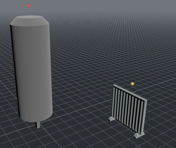
For a simple example, you have a water heater connected to a radiator. Your virtual model gets data from the heater’s sensors and knows the temperature of the heater. The radiator on the other hand has no sensor attached to it. But the link between the heater and 3D picture of water heater and radiatorradiator is in your digital model. Now you can see virtually that when the heater is malfunctioning, your radiator gets colder. Not only sensors are connected to your digital twin, but manuals and other documents are also. So you can view the heater’s manual right there in the dashboard.

Industrial point of view benefits

We are living in an age when everything is connected to the internet and industrial devices are no different. Huge amounts of data is flowing from devices to different endpoints. That’s where digital twins will show its strengths by connecting all those dots to form a bigger picture about process and assets. Making it easier to understand complex structures. It’s also a two-way street, so digital twins can generate more useful data or update existing data.

Many times industrial processes consist of other processes that aren’t connected to each other. Like that lonely motor spinning without real connection to other parts of the process. Those are easily forgotten, even if it is a crucial part of the process. When complexity grows there will be even more loose ends that aren’t connected to each other.

  • Predictive maintenance lowers maintenance costs.
  • Productivity will improve, because reduced downtime and improved performance via optimization.
  • Testing in the digital world before real world applications.
  • Allows you to make more informed decisions at the beginning of the process.
  • Continuous improvement through simulations.

Digital twins offer great potential for predicting the future instead of analyzing the past. Real world experiments aren’t a cost effective way to test ideas. With a digital counterpart you can cost effectively test ideas and see if you missed something important.

Quick overview of creating digital twins with AWS IoT Twinmaker

In workspace you create entities that are digital versions of devices. Those entities are connected with components that will handle data connections. Components can connect to AWS Sitewise or other data source via AWS lambda. When creating a component you define it in JSON format and it can inherit other components.

Next step is to get your CAD models uploaded to the Twinmaker. When you have your models uploaded, you can start creating 3D scenes that will visualize your digital twin. Adding visual rules like tags that change their appearance can be done in this phase.

Now digital twin is almost ready and the only thing to do is connect Grafana with Twinmaker and create a dashboard in Grafana. Grafana has a plugin for Twinmaker that helps with connecting 3D scenes and data.

There are many other tools for creating digital twins and what to use, depends on the needs.

If you are interested in how to create Digital Twins please reach out to me or the Solita Industrial team. Please also check our kickstart for Connected Factory and blog posts related to Smart and Connected Factories


SQL Santa for Factory and Fleet

Awesome SQL Is coming To Town

We have a miniseries before Christmas coming where we talk S-Q-L, /ˈsiːkwəl/ “sequel”. Yes, the 47 years old domain-specific language used in programming and designed for managing data. It’s very nice to see how old faithful SQL is going stronger than ever for stream processing as well the original relational database management purposes.

What is data then and how that should be used ? Take a look on article written in Finnish “Data ei ole öljyä, se on lantaa”

We will show you how to query and manipulate data across different solutions using the same SQL programming language.

The Solita Developer survey has become a tradition here at Solita and please check out the latest survey. It’s easy to see how SQL is dominating in a pool of many cool programming languages. It might take an average learner about two to three weeks to master the basic concepts of SQL and this is exactly what we will do with you.

Data modeling and real-time data

Operative technology (OT) solution have been real time from day one despite it’s also a question of illusion of real-time when it comes to IT systems. We could say that having network latency 5-15 ms towards Cloud and data processing with single-digit millisecond latency irrespective of the scale is considered near real time. This is important for Santa Claus and Industry 4.0 where autonomous fleet, robots and real-time processing in automation and control is a must have. Imagine situation where Santa’s autonomous sleigh with smart safety systems boosted computer vision (CV) able bypass airplanes and make smart decisions would have time of unit seconds or minutes – that would be a nightmare.

A data model is an abstract model that organizes elements of data and standardizes how they relate to one another and to the properties of real-world entities.

It’s easy to identify at least conceptual, logical and physical data models, where from the last one we are interested the most in this exercise to store and query data.

Back to the Future

Dimensional model heavily development by Ralph Kimball was breakthrough 1996 and had concepts like fact tables, dimension and ultimately creating a star schema. Challenge of this modeling is to keep conformed dimensions across the data warehouse and data processing can create unnecessary complexity.

One of the main driving factors behind using Data Vault is for both audit and historical tracking purposes. This methodology was developed by Daniel (Dan) Linstedt in early 2000. It has gain a lot of attraction being able to support especially modern cloud platform with massive parallel processing (MPP) of data loading and not to worry so much of which entity should be loaded first. Possibility even create data warehouse from scratch and just loading data in is pretty powerful when designing an idempotent system. 

Quite typical data flow looks like picture above and like you already noticed this will have impact on how fast data is landed into applications and users. Theses for Successful Modern Data Warehousing are useful to read when you have time.

Data Mesh ultimate promise is to eliminate the friction to deliver quality data for producers and enable consumers to discover, understand and use the data at rapid speed. You could imagine this as data products in own sandboxes with some common control plane and governance. In any case to be successful you need expertise from different areas such as business, domain and data. End of the day Data Mesh does not take a strong position on data modeling.

Wide Tables / One Big Table (OBT) that is basically nested and denormalized tables is one modeling that is perhaps the mostly controversy. Shuffling data between compute instances when executing joins will have negative impact on performance (yes, you can e.g. replicate dimensional data to nodes and keep fact table distributed which will improve performance) and very often operational data structures produced by micro-services and exchanged over API are closer to this “nested” structure. Having same structure and logic for batch SQL as streaming SQL will ease your work.

Breaking down the OT data items to multiple different sub optimal data strictures inside IT systems will loose the single, atomic data entity. Having said this it’s possible to ingest e.g. Avro files to MPP, keeping the structure same as original file as and using evolving schemas to discovery new attributes. That can be then use as baseline to load target layers such as Data Vault.

One interesting concept called Activity Schema that is sold us as being designed to make data modeling and analysis substantially simpler, faster.

Contextualize data

For our industrial Santa Claus case one very important thing is how to create inventory and contextualize data. One very promising path is an augmented data catalog that will cover a bit later. For some reason there is material out there explaining how IoT data has no structure which is just incorrect. The only reason I can think is that kind of data asset was not fit to traditional data warehouse thinking.

Something to take a look is Apache Avro that is a language-neutral data serialization system, developed by Doug Cutting, the father of Hadoop. The other one is JSON is an open standard file format and data interchange format that uses human-readable text to store and transmit data objects consisting of attribute–value pairs and arrays. This is not solution for data modeling even more you will notice later on this blog post how those are very valuable on steaming data and having schema compared to other formats like CSV.

Business case for Santa

Like always everything starts with Why and solution discovery phase, what we actual want to build and would that have a business value. At Christmas time our business is around gifts and how to deliver those on time. Our model is a bit more simplified and will include operational technology systems such as assets (Santa’s workshop) and fleet (sleighs) operations. There might always be something broken so few maintenance needs are pushed to technicians (elfs). Distributed data platform is used for supply chain and logistics analytics to remove bottlenecks so business owners can be satisfied (Santa Claus and the team) and all gifts will be delivered to the right address just in time.

Case Santa’s workshop

We can later use OEE to calculate that workshop performance in order to produce high quality nice gifts. Data is ingested real time and contextualized so once a while Santa and the team will check how we are doing. In this specific case we know that using Athena we can find relevant production line data just querying the S3 bucket where all raw data is stored already.

Day 1 – creating a Santa’s table for time series data

Let’s create a very basic table to capture all data from Santa’s factory floor. You will notice there are different data types like bigint and string. You can even add comments to help others to later find what kind of data field should include. In this case raw data is Avro but you do not have to worry about that so let’s go.

CREATE EXTERNAL TABLE `raw`(

`seriesid` string COMMENT 'from deserializer',

`timeinseconds` bigint COMMENT 'from deserializer',

`offsetinnanos` bigint COMMENT 'from deserializer',

`quality` string COMMENT 'from deserializer',

`doublevalue` double COMMENT 'from deserializer',

`stringvalue` string COMMENT 'from deserializer',

`integervalue` int COMMENT 'from deserializer',

`booleanvalue` boolean COMMENT 'from deserializer',

`jsonvalue` string COMMENT 'from deserializer',

`recordversion` bigint COMMENT 'from deserializer'

) PARTITIONED BY (

`startyear` string, `startmonth` string,

`startday` string, `seriesbucket` string

)

Day 2 – query Santas’s data

Now we have a table and how to query that one ? That is easy with SELECT and taking all fields using asterix. It’s even possible to limit that to 10 rows which is always a good practice.

SELECT * FROM "sitewise_out"."raw" limit 10;

Day 3 – Creating a view from query

View is a virtual presentation of data that will help to organize assets more efficiently. One golden rule is still now to create many views on top of other views and keep the solution simple. You will notice that CREATE VIEW works nicely and now we have timeinseconds and actual factory floor value (doublevalue) captured. You can even drop the view using DROP command.

CREATE OR REPLACE VIEW "v_santa_data"

AS SELECT timeinseconds, doublevalue FROM "sitewise_out"."raw" limit 10;

Day 4 – Using functions to format dates to Santa

You noticed that timeinseconds is in Epoch so let’s use functions to have more human readable output. So we add a small from_unixtime function and combine that with date_format to have formatted output like we want. Perfect, now we know from which data Santa Claus manufacturing data originated.

SELECT date_format(from_unixtime(timeinseconds),'%Y-%m-%dT%H:%i:%sZ') , doublevalue FROM "sitewise_out"."raw" limit 10;

 Day 5 – CTAS creating a table

Using CTAS (CREATE TABLE AS SELECT) you can even create a new physical table easily. You will notice that Athena specific format has been added that you do not need on relational databases.

CREATE TABLE IF NOT EXISTS new_table_name

WITH (format='Avro') AS

SELECT timeinseconds , doublevalue FROM "sitewise_out"."raw" limit 10;

Day 6 – Limit the result sets

Now I want to limit the results to only those where the quality is Good.Adding a WHERE clause I can have only those rows printed to my output – that is cool!

SELECT * FROM "sitewise_out"."raw"  where quality='GOOD' limit 10;


Case Santa’s fleet

Now we jump into Santa’s fleet meaning sleights and there is few attribute we are interested like SleightD , IsSmartLock, LastGPSTime , SleightStateIDLatitude and Longitude. This data is time series that is ingested into our platform near real-time. Let’s use AWS Timestream service which is fast, scalable, and serverless time series database service for IoT and operational applications. A time series is a data set that tracks a sample over time. 

Day 7 – creating a table for fleet

You will notice very quickly that data model looks different than on relational database cases. There is no need beforehand to define table structure just executing CreateTable is enough.


Day 8- query the latest record

You can override time field using e.g. LastGPSTime, in this example we use time when data was ingested in, so getting the last movement of sleigh would be like this.

SELECT * FROM movementdb.tbl_movement
ORDER BY time DESC
LIMIT 1

Day 9- let’s check the last 24 hours movement

We can use time to filter our results and ordering on descending same time.

SELECT *
FROM "movementdb"."tbl_movement" 
WHERE time > ago(24h) 
ORDER BY time DESC

Day 10- latitude and longitude

We can find out latitude and longitude information easily and please note we are using IN operator to bet both to query result.

SELECT measure_name,measure_value::double,time 
FROM "movementdb"."tbl_movement" 
WHERE time > ago(24h) 
and measure_name in ('Longitude','Latitude')
ORDER BY time DESC LIMIT 10

Day 11- last connectivity info

Now we use 2 things so we group data based on sleigh id and find the maximum value. This will tell when sleigh was connected and sending data to our platform. There are plenty of functions to choose from so please check documentation.

SELECT greatest (time) as last_time, sleighId
FROM "movementdb"."tbl_movement" 
WHERE time > ago(24h) 
and measure_name = ('LastGPSTime')
group by sleighId,greatest (time)

Day 12- using conditions for smart lock data

CASE is very powerful to manipulate the query results so in this example we use that do indicate better if sleigh had smart lock.

SELECT time, measure_name,
CASE 
WHEN measure_value::boolean = true THEN 'Yes we have a smart lock'
ELSE 'No we do not that kind of fancy locks'
END AS smart_lock_info
FROM "movementdb"."tbl_movement"
WHERE time between ago(1d) and now() 
and measure_name='IsSmartLock'

Day 13- finding the latest battery level on each fleet equipment

This would be a bit more complex so we have one query to find max value of battery level and then we later join that to base data so on each record we know the latest battery level in the past 24 hours. Please notice we are using INNER join in this example.

WITH latest_battery_time as (
select 
d_sleighIdentifier, 
max(time) as latest_time 
FROM 
"movementdb"."tbl_movement" 
WHERE 
time between ago(1d) 
and now() 
and measure_name = 'Battery' 
group by 
d_sleighIdentifier
) 
SELECT 
b.d_sleighIdentifier, 
b.measure_value :: double as last_battery_level 
FROM 
latest_battery_time a 
inner join "movementdb"."tbl_movement" b on a.d_sleighIdentifier = b.d_sleighIdentifier 
and b.time = a.latest_time 
WHERE 
b.time between ago(1d) 
and now() 
and b.measure_name = 'Battery'

Day 14- distinct values

The SELECT DISTINCT statement is used to return only distinct (different) values. This is so create and also very misused when removing duplicates etc. when actual problem can be on JOIN conditions.

SELECT 
DISTINCT (d_sleighIdentifier) 
FROM 
"movementdb"."tbl_movement"

Day 15- partition by is almost magic

The PARTITION BY clause is a subclause of the OVER clause. The PARTITION BY clause divides a query’s result set into partitions. The window function is operated on each partition separately and recalculate for each partition. This is almost a magic and that can be used in several ways like in this example identify last sleigh Id.

select 
d_sleighIdentifier, 
SUM(1) as total, 
from 
(
SELECT 
*, 
first_value(d_sleighIdentifier) over (
partition by d_sleighTypeName 
order by 
time desc
) lastaction 
FROM 
"movementdb"."tbl_movement" 
WHERE 
time between ago(1d) 
and now()
) 
GROUP BY 
d_sleighIdentifier, 
lastaction

Day 16- interpolation (values of missing data points)

Timestream and few other IoT services supports linear interpolation, enabling to estimate and retrieve the values of missing data points in their time series data. This will come very handy when our fleet is not connected all the time, in this example we used it for our smart sleight battery level.

WITH rawseries as (
select 
measure_value :: bigint as value, 
time as d_time 
from 
"movementdb"."tbl_movement" 
where 
measure_name = 'Battery'
), 
interpolate as (
SELECT 
INTERPOLATE_LINEAR(
CREATE_TIME_SERIES(d_time, value), 
SEQUENCE(
min(d_time), 
max(d_time), 
1s
)
) AS linear_ts 
FROM 
rawseries
) 
SELECT 
time, 
value 
FROM 
interpolate CROSS 
JOIN UNNEST(linear_ts)

Case Santa’s  master data

Now we jump into Master Data when factory and fleet is up are covered. In this very complex supply chain system customer data is very typical transactional data and in this exercise we keep it very atomic having stored only very basic info into DynamoDB that is a fully managed, serverless, key-value NoSQL database designed to run high-performance applications at any scale. We use this data to on IoT data streams for join, filtering and other purposes in fast manner. Good to remember that DynamoDB is not build for complex query patterns so it’s best on it’s original key=value data query pattern.

Day 17- adding master data

We upload our customer data into DynamoDB so called “items” based om the list received from Santa.

{
"customer_id": {
"S": "AJUUUUIIIOS"
},
"category_list": {
"L": [
{
"S": "Local Businesses"
},
{
"S": "Restaurants"
}
]
},
"homepage_url": {
"S": "it would be here"
},
"founded_year": {
"N": "2021"
},
"contract": {
"S": "NOPE"
},
"country_code": {
"S": "FI"
},
"name": {
"S": ""
},
"market_stringset": {
"SS": [
"Health",
"Wellness"
]
}
}

Day 18- query one customer item

Amazon DynamoDB supports PartiQL, a SQL-compatible query language, to select, insert, update, and delete data in Amazon DynamoDB. That is something we will use too speed up things. Let’s first query one customer data asset.

SELECT * FROM "tbl_customer" where customer_id='AJUUUUIIIOS'

Day 18- update kids information

Using the same PartiQL you can update item to have new attributes with one go.

UPDATE "tbl_customer" 
SET kids='2 kids and one dog' 
where customer_id='AJUUUUIIIOS'

Day 19- contains function

Now we can easily check that form marketing data who was interested on Health using CONTAINS. Many moderns database engines have native support for semi-structured data, including: Flexible-schema data types for loading semi-structured data without transformation. If you are not already familiar please take a look on AWS Redshift and Snowflake.

SELECT * FROM "tbl_customer" where contains("market_stringset", 'Health')

Day 20- inserting a new customer

Using familiar SQL like it’s very straightforward to add one new item.

INSERT INTO "tbl_customer" value {'name' : 'name here','customer_id' : 'A784738H'}

Day 21- missing data

Using a special MISSING you can find those where some attribute is not present easily.

SELECT * FROM "tbl_customer" WHERE "kids" is MISSING

Day 22- export data into s3

With one command you can export data from DynamoDB to S3 so let’s do that one based on documentation. AWS and others do have support for something called Federated Query where you can run SQL queries across data stored in relational, non-relational, object, and custom data sources. This federated feature we will cover later with You.

Day 23- using S3 select feature

Now you have data stored to  S3 bucket and there is holder called /data so you can even use SQL to query S3 stored data. This will find relevant information for customer_id.

Select s.Item.customer_id from S3Object s

Day 24- s3 select to find right customer

You can even use customer Id to restrict data returned to you.

Select s.Item.customer_id from S3Object s where s.Item.customer_id.S ='AJUUUUIIIOS'


That’s all, I hope you get some glimpse how useful SQL is even you have different services and you might first think this will never be possible to use same kind of language of choice. Please do remember when some day You might be building next generation artificial intelligence and analysis platform with us knowing few data modeling techniques and SQL is a very good start.

You might be interested Industrial equipment data at scale for factory floor or manage your fleet at scale so let’s keep fresh mind and have a very nice week !

 

AWS SageMaker Pipelines – Making MLOps easier for the Data Scientist

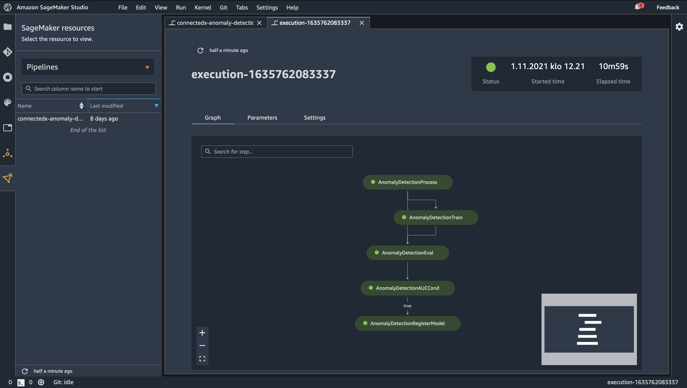
SageMaker Pipelines is a machine learning pipeline creation SDK designed to make deploying machine learning models to production fast and easy. I recently got to use the service in an edge ML project and here are my thoughts about its pros and cons. (For more about the said project refer to Solita data blog series about IIoT and connected factories https://data.solita.fi/factory-floor-and-edge-computing/)

Example pipeline

Why do we need MLOps?

First, there were statistics then came the emperor’s new clothes – machine learning, a rebranding of old methods accompanied with new ones emerged. Fast forward to today and we’re all the time talking about this thing called “AI”, the hype is real, it’s palpable because of products like Siri and Amazon Alexa.

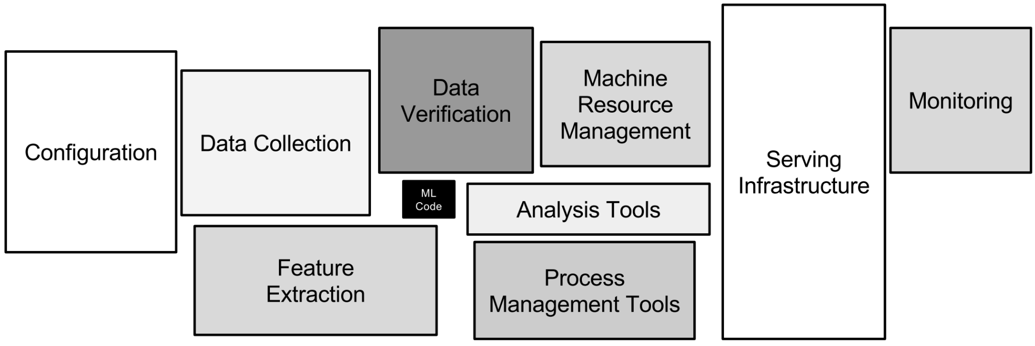
But from a Data Scientist point of view, what does it take to develop such a model? Or even a simpler model, say a binary classifier? The amount of work is quite large, and this is only the tip of the iceberg. How much more work is needed to put that model into the continuous development and delivery cycle?

For a Data Scientist, it can be hard to visualize what kind of systems you need to automate everything your model needs to perform its task. Data ETL, feature engineering, model training, inference, hyperparameter optimization, performance monitoring etc. Sounds like a lot to automate?

(Hidden technical debt in machine learning https://proceedings.neurips.cc/paper/2015/file/86df7dcfd896fcaf2674f757a2463eba-Paper.pdf)


This is where MLOps comes to the picture, bridging DevOps CI/CD practices to the data science world and bringing in some new aspects as well. You can see more information about MLOps from previous Solita content such as https://www.solita.fi/en/events/webinar-what-is-mlops-and-how-to-benefit-from-it/ 

Building an MLOps infrastructure is one thing but learning to use it fluently is also a task of its own. For a Data Scientist at the beginning of his/her career, it could seem too much to learn how to use cloud infrastructure as well as learn how to develop Python code that is “production” ready. A Jupyter notebook outputting predictions to a CSV file simply isn’t enough at this stage of the machine learning revolution.

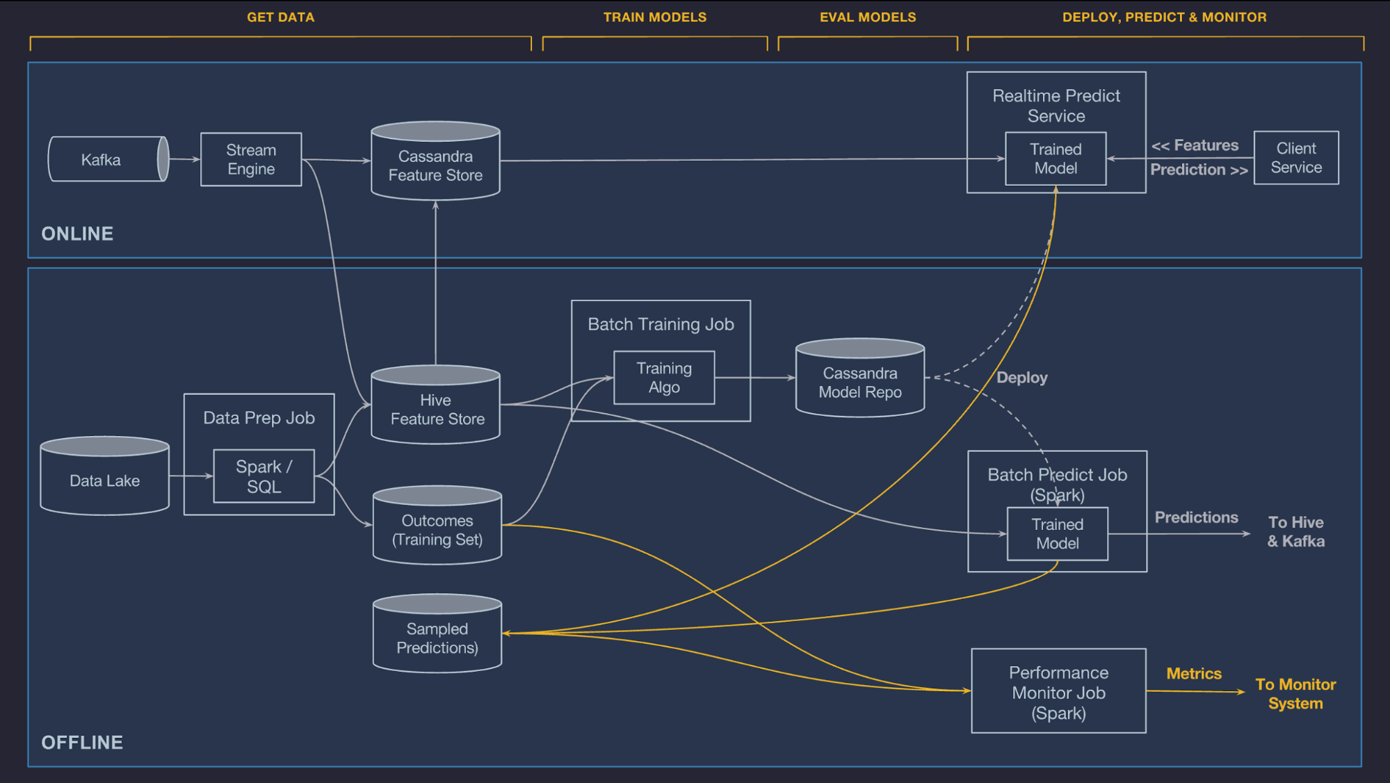
(The “first” standard on MLOps, Uber Michelangelo Platform https://eng.uber.com/michelangelo-machine-learning-platform/)


A Jupyter notebook outputting predictions to a CSV file simply isn’t enough at this stage of the machine learning revolution.

Usually, companies that have a long track record of Data Science projects have a few DevOps, Data Engineer/Machine Learning Engineer roles working closely with their Data Scientists teams to distribute the different tasks of production machine learning deployment. Maybe they even have built the tooling and the infrastructure needed to deploy models into production more easily. But there are still quite a few Data Science teams and data-driven companies figuring out how to do this MLOps thing.

Why should you try SageMaker Pipelines?

AWS is the biggest cloud provider ATM so it has all the tooling imaginable that you’d need to build a system like this. They are also heavily invested in Data Science with their SageMaker product and new features are popping up constantly. The problem so far has been that there are perhaps too many different ways of building a system like this.

AWS tries to tackle some of the problems with the technical debt involving production machine learning with their SageMaker Pipelines product. I’ve recently been involved in project building and deploying an MLOps pipeline for edge devices using SageMaker Pipelines and I’ll try to provide some insight on why it is good and what is lacking compared to a completely custom-built MLOps pipeline.

The SageMaker Pipelines approach is an ambitious one. What if, Data Scientists, instead of having to learn to use this complex cloud infrastructure, you could deploy to production just by learning how to use a single Python SDK (https://github.com/aws/sagemaker-python-sdk)? You don’t even need the AWS cloud to get started, it also runs locally (to a point).

SageMaker Pipelines aims at making MLOps easy for Data Scientists. You can define your whole MLOps pipeline in f.ex. A Jupyter Notebook and automate the whole process. There are a lot of prebuilt containers for data engineering, model training and model monitoring that have been custom-built for AWS. If these are not enough you can use your containers enabling you to do anything that is not supported out of the box. There are also a couple of very niche features like out-of-network training where your model will be trained in an instance that has no access to the internet mitigating the risk of somebody from the outside trying to influence your model training with f.ex. Altered training data.

You can version your models via the model registry. If you have multiple different use cases for the same model architectures with differences being in the datasets used for training it’s easy to select the suitable version from SageMaker UI or the python SDK and refactor the pipeline to suit your needs.  With this approach, the aim is that each MLOps pipeline has a lot of components that are reusable in the next project. This enables faster development cycles and the time to production is reduced. 

SageMaker Pipelines logs every step of the workflow from training instance sizes to model hyperparameters automatically. You can seamlessly deploy your model to the SageMaker Endpoint (a separate service) and after deployment, you can also automatically monitor your model for concept drifts in the data or f.ex. latencies in your API. You can even deploy multiple versions of your models and do A/B testing to select which one is proving to be the best.

And if you want to deploy your model to the edge, be it a fleet of RaspberryPi4s or something else, SageMaker provides tooling for that also and it seamlessly integrates with Pipelines.

You can recompile your models for a specific device type using SageMaker Neo Compilation jobs (basically if you’re deploying to an ARM etc. device you need to do certain conversions for everything to work as it should) and deploy to your fleet using SageMaker fleet management.

Considerations before choosing SageMaker Pipelines

By combining all of these features to a single service usable through SDK and UI, Amazon has managed to automate a lot of the CI/CD work needed for deploying machine learning models into production at scale with agile project development methodologies. You can also leverage all of the other SageMaker products f.ex. Feature Store or Forekaster if you happen to need them. If you’re already invested in using AWS you should give this a try.

Be it a great product to get started with machine learning pipelines it isn’t without its flaws. It is quite capable for batch learning settings but there is no support as of yet for streaming/online learning tasks. 

And for the so-called Citizen Data Scientist, this is not the right product since you need to be somewhat fluent in Python. Citizen Data Scientists are better off with BI products like Tableau or Qlik (which use SageMaker Autopilot as their backend for ML) or perhaps with products like DataRobot. 

And in a time where software products are high availability and high usage the SageMaker EndPoints model API deployment scenario where you have to pre-decide the number of machines serving your model isn’t quite enough.

 In e-commerce applications, you could run into situations where your API is receiving so much traffic that it can’t handle all the requests because you didn’t select a big enough cluster to serve the model with. The only way to increase the cluster size in SageMaker Pipelines is to redeploy a new revision within a bigger cluster. It is pretty much a no brainer to use a Kubernetes cluster with horizontal scaling if you want to be able to serve your model as the traffic to the API keeps increasing.

Overall it is a very nicely packaged product with a lot of good features. The problem with MLOps in AWS has been that there are too many ways of doing the same thing and SageMaker Pipelines is an effort for trying to streamline and package all those different methodologies together for machine learning pipeline creation.

It’s a great fit if you work with batch learning models and want to create machine learning pipelines really fast. If you’re working with online learning or reinforcement models you’ll need a custom solution. And if you are adamant that you need autoscaling then you need to do the API deployments yourself, SageMaker endpoints aren’t quite there yet. For references to a “complete” architecture refer to the AWS blog https://aws.amazon.com/blogs/machine-learning/automate-model-retraining-with-amazon-sagemaker-pipelines-when-drift-is-detected/


Factory Floor and Edge computing

Happened last time

In the first part of this blog series I discussed the industry 4.0 phenomenon: Smart and Connected Factory, what benefits it brings, what is IT/OT convergence and gave a short intro about Solita’s Connected Factory Kickstart

This part is more focused on the data at Factory floor and how AWS services can help in ingesting the data from factory machinery.

Access the data and gain benefits from Edge computing

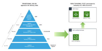
So what is the data at the Factory floor? It is generated by machinery systems using many sensors and actuators. See the following picture where on the left there is a traditional ISA-95 pyramid for factory data integrating each layer with the next. The right side represents new thinking where we can ingest data from each layer and take advantage of IT/OT convergence using AWS edge and cloud services.

PLC (Programmable Logic Controller) typically has dedicated modules for inputs and dedicated modules for outputs. An input module can detect the status of input signals like switches and an output module controls devices such as relays and motors.

Sensors are typically connected to PLC’s. To access the data and use it in other systems, PLC’s can be connected to an OPC-UA server. The server can provide access to the data. One traditional use case is to connect PLC to factory SCADA systems for high level supervision of machines and processes. OPC-UA defines a generic object model and each object can be associated with data type, timestamp, data quality and current value and they can have a hierarchy. Every kind of device, function, and system information can be described using this meta model.


AWS services that ease data access at the factory

AWS Greengrass is an open source edge software which integrates to AWS Cloud. It enables local processing, messaging, Machine Learning (ML) inference, device mesh and many pre-baked software components for speed up application development. 

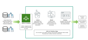
AWS Sitewise is a cloud service for collecting and analyzing data from factory environments. It provides Greengrass compatible edge components for example for data collection from OPC-UA server and for streaming data to AWS Sitewise. Sitewise has a built in time-series database, data modeling capabilities, API layer and portal, which can be deployed and run at the edge as well (which is amazing!). 

The AWS Sitewise asset and data modeling is for making a virtual presentation of industrial equipment or process. Data model supports hierarchies, metrics and real time calculations, for example for calculating OEE (Overall Equipment Effectiveness). Each asset is enforced to use data mode that validates incoming data and schema.

Why industrial use cases with AWS?

I prefer more hands-on work than reading Gartner papers; anyhow AWS has been named as a Leader for the eleventh consecutive year and has secured the highest and furthest position on the ability to execute and completeness of vision axes in the 2021 Magic Quadrant for Cloud Infrastructure and Platform Services. It’s very nice to see how AWS is taking industrial solutions seriously and packaging those to a model that is easy to take in use for building digital services to the factory floor and cloud.  

 1. AWS Sitewise – The power of data model, ingest, analyze and visualize

Sitewise packages nice features which I feel are the greatest are the data and asset modeling, near real time metric calculations (even on edge), visualization and build in time series database. Sitewise is nicely supported by CloudFormation, so you can automate the deployment and even build data models according to your OPC-UA data model automatically (Meta driven Industry standard data model). The Fact that there are edge processing and monitoring capabilities with a portal available makes the Sitewise a really competitive package.

2. AWS Greengrass – Edge computing and secure cloud integration

Speeds up edge application development with public components, like the OPC-UA collector, StreamManager and Kinesis Firehose publisher. The latest Greengrass version 2.x has evolved and has lots of great features. You can provision and run a solution on real hardware or simulate on an EC2 instance or Docker, as you wish. One way to provision Greengrass devices to AWS cloud is to use IoT Fleet Provisioning, where certificates for the device are created on the first connection attempt to the cloud. Applications are easy to deploy from cloud IoT Core to edge Greengrass instances. You can also run serverless AWS Lambdas at the edge, which is really superb! All in all, the complete Greengrass 2.0 package will speed up development.

3. Cloud and Edge – Extra layer of Security

SItewise and Greengrass use AWS IoT Core security features, like certificate based authentication, IoT policies, TLS 1.2 on transport and device defender, which brings the security to a new level. It’s also possible to use custom Certificate Authorities (CA) to issue edge device certificates. Custom CA’s can be stored in AWS CloudHSM and AWS Certificate Manager. Now I can really say that security is our best friend.

4. Agile integration to other solutions

Easy way for integrating data to other solutions is to use Sitewise Edge and Cloud APIs. If you deploy Sitewise to the edge the API is usable there as well, and you can use the data for other factory systems, like MES (Manufacturing Execution System). At least I think this will combine the IT and OT worlds like never before.

5. AutoML for Edge computing

AutoML is for people like me and citizen data scientists, something that will speed up business insights when creating a lot of notebooks or python code is not needed anymore.

These AutoML services are used to organize, track and compare Machine Learning training. When auto deploy is turned on the best model from the experiment is deployed to the endpoint and the best model is automatically selected using the Bandit algorithm. Besides these Amazon SageMaker model monitor will continuously monitor the quality of your machine learning models in real time and I can focus on talking with people and not only machines. 


Stay tuned for more

I think that AWS is making it easier to combine cloud workloads with edge computing. Stay tuned for the next blog post where we dig more into the cloud side of this, including Sitewise, Asset and data model, visualization and alarms. And please take a look at the “Predictive maintenance data kickstart” if you haven’t yet:

https://www.solita.fi/en/solita-connected/


Smart and Connected Factories

Smart connected factories are a phenomenon of the fourth industrial revolution, Industry 4.0.

What is a connected factory?

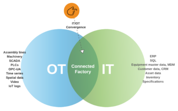
Connected Factories utilizes machinery automation systems and additional sensors to collect data from manufacturing devices and processes. The data can be analyzed and processed on site at the factory, before being sent to the cloud platforms for historical and real time data analysis. Connected factory enables a holistic view for data over all customer factories. Connectivity is a key enabler of  IT/OT convergence.

Operational Technology (OT) consists of software and hardware systems that control and execute processes at the factory floor. Typically these are MES (Manufacturing Execution System), SCADA (Supervisory Control And Data Acquisition) and PLCs (Programmable Logic Controllers) at manufacturing factories. 

Whereas Information Technology (IT) refers to the information infrastructure covering network, software and hardware components for storing, processing, securing and exchanging data. IT consists of laptops and servers, software, enterprise systems software like ERPs, CRMs, inventory management programs, and other business related tools.

Historically OT is separated from IT. In recent years industrial digitalization, connectivity and cloud computing have made it possible for OT and IT systems to join and share data with each other. On IT/OT data convergence factory floor OT data is combined with IT data:

IT/OT Convergence
IT/OT Convergence


When IT and OT collide we need to align things like “How to handle different networks and control the boundaries between them”. IT and OT networks are totally for different purposes and they have different security, availability and maintainability principles. IT/OT convergence can definitely be beneficial for the company but at the same time it might pop up new challenges for the traditional OT world, like “How often and what kind of data should we upload to the cloud?” and “What are the key attributes to combine different data assets?”. Here are few examples where IT/OT is  converged:

  • Welding station monitoring with laboratory data. Combining with IT data we can improve customer specific welding quality. 
  • Getting OT data from equipment and merging that with customer contract data we can start upselling predictive maintenance solutions.
  • Getting real time metrics it is also possible to create subscription based billing. For this we need asset basic information and CRM customer contract information.
  • Creating a Digital service book is easy when you have full traceability based on OT data joint to IT product lifecycle data.

I think that in order to combine IT and OT together is nowadays much easier than just a few years ago thanks to hyper scalers like AWS and others. Now we can see in action how Cloud can enable smart manufacturing using purpose built components like AWS Greengrass and SiteWise. Stay tuned for next blog posts where I will explain basics on Edge computing in a harsh factory environment.


Kickstart towards smart and connected factory

Solita has made a kickstart for companies to start a risk free journey. We package pre-baked components for edge data ingestion, edge ML, AWS Sitewise data modelling, visualization, data integration API and MLOps in one deliverable using only 4 weeks time.

Check it out from https://www.solita.fi/en/solita-connected/ and let’s connect!