Pyspark looks like regular python code, but the distributed nature of the execution requires the whole new way of thinking to optimize the code.

PySpark execution logic and code optimization

PySpark looks like regular python code. In reality the distributed nature of the execution requires the whole new way of thinking to optimize the PySpark code.

This article will focus on understanding PySpark execution logic and performance optimization. PySpark DataFrames are in an important role.

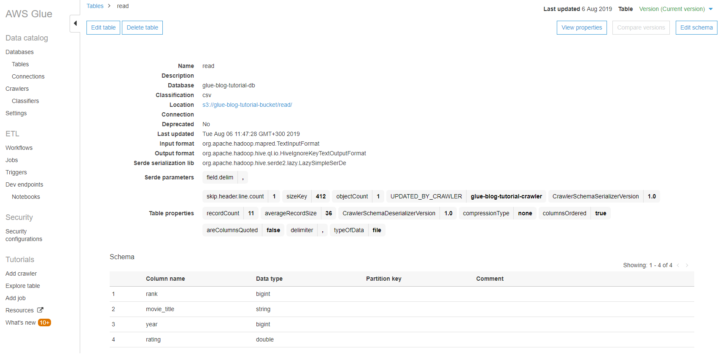
To try PySpark on practice, get your hands dirty with this tutorial: Spark and Python tutorial for data developers in AWS

DataFrames in pandas as a PySpark prerequisite

PySpark needs totally different kind of engineering compared to regular Python code.

If you are going to work with PySpark DataFrames it is likely that you are familiar with the pandas Python library and its DataFrame class.

Here comes the first source of potential confusion: despite their similar names, PySpark DataFrames and pandas DataFrames behave very differently. It is also easy to confuse them in your code. You might want to use suffix like _pDF for pandas DataFrames and _sDF for Spark DataFrames.

The pandas DataFrame object stores all the data represented by the data frame within the memory space of the Python interpreter. All of the data is easily and immediately accessible. The operations on the data are executed immediately when the code is executed, line by line. It is easy to print intermediate results to debug the code.

However, these advantages are offset by the fact that you are limited by the local computer’s memory and processing power constraints – you can only handle data which fits into the local memory. But since the operations are done in memory, with a basic data processing task you do not need to wait more than a few minutes at maximum.

PySpark DataFrames and their execution logic

The PySpark DataFrame object is an interface to Spark’s DataFrame API and a Spark DataFrame within a Spark application. The data in the DataFrame is very likely to be somewhere else than the computer running the Python interpreter – e.g. on a remote Spark cluster running in the cloud.

There are two distinct kinds of operations on Spark DataFrames: transformations and actions. Transformations describe operations on the data, e.g. filtering a column by value, joining two DataFrames by key columns, or sorting data. Actions are operations which take DataFrame(s) as input and output something else. Some examples from action would be showing the contents of a DataFrame or writing a DataFrame to a file system.

The key point to understand how Spark works is that transformations are lazy. Executing a Python command which describes a transformation of a PySpark DataFrame to another does not actually require calculations to take place. Ordering by a column and calculating aggregate values, returning another PySpark DataFrame would be such transformation. Rather, the operation is added to the graph describing what Spark should eventually do.

When an action is requested – e.g. return the contents of this Spark DataFrame as a Pandas DataFrame – Spark looks at the processing graph and then optimizes the tasks which needs to be done. This is the job of the Catalyst optimizer, and it enables Spark to optimize the operations to very high degree.

Also, the actual computation tasks run on the Spark cluster, meaning that you can have huge amounts of memory and processing cores available for the actual computation, even without resorting to the top-of-the-line virtual machines offered by cloud providers.

Consider caching to speed up PySpark

However, the highly optimized and parallelized execution comes at a cost: it is not as easy to see what is going on at each step. Looking at the data after some transformations means that you have to gather the data, or its subset, to a single computer. This is an action, so Spark has to determine the computation graph, optimize it, and execute it.

If your dataset is large, this may take quite some time. This is especially true if caching is not enabled and Spark has to start by reading the input data from a remote source – such as a database cluster or cloud object storage like S3.

You can alleviate this by caching the DataFrame at some suitable point. Caching causes the DataFrame partitions to be retained on the executors and not be removed from memory or disk unless there is a pressing need. In practice this means that the cached version of the DataFrame is available quickly for further calculations. However, playing around with the data is still not as easy or quick as with pandas DataFrames.

Use small scripts and multiple environments in PySpark

As a rule of thumb, one PySpark script should perform just one well defined task. This is due to the fact that any action triggers the transformation plan execution from the beginning. Managing and debugging becomes a pain if the code has lots of actions.

The normal flow is to read the data, transform the data and write the data. Often the write stage is the only place where you need to execute an action. Instead of debugging in the middle of the code, you can review the output of the whole PySpark job.

With large amounts of data this approach would be slow. You would have to wait a long time to see the results after each job.

My suggestion is to create environments that have different sizes of data. In the environment with little data you test the business logic and syntax. The test cycle is rapid as there’s no need process gigabytes of data. Running the PySpark script with the full dataset reveals the performance problems.

This goes well together with the traditional dev, test, prod environment split.

Favor DataFrame over RDD with structured data

RDD (Resilient Distributed Dataset) can be any set of items. For example, a shopping list.

["apple", "milk", "bread"]

RDD is the low-level data representation in Spark, and in earlier versions of Spark it was also the only way to access and manipulate data. However, the DataFrame API was introduced as an abstraction on top of the RDD API. As a rule of thumb, unless you are doing something very involved (and you really know what you are doing!), stick with the DataFrame API.

DataFrame is a tabular structure: a collection of Columns, each of which has a well defined data type. If you have a description and amount for each item in the shopping list, then a DataFrame would do better.

+-------+-----------+------+
|product|description|amount|
+-------+-----------+------+
|apple  |green      |5     |
|milk   |skimmed    |2     |
|bread  |rye        |1     |
+-------+-----------+------+

This is also a very intuitive representation for structured data, something that can be found from a database table. PySpark DataFrames have their own methods for data manipulation just like pandas DataFrames have.

Avoid User Defined Functions in PySpark

As a beginner I thought PySpark DataFrames would integrate seamlessly to Python. That’s why I chose to use UDFs (User Defined Functions) to transform the data.

A UDF is simply a Python function which has been registered to Spark using PySpark’s spark.udf.register method.

With the small sample dataset it was relatively easy to get started with UDF functions. When running the PySpark script with more data, spark popped an OutOfMemory error.

Investigating the issue revealed that the code could not be optimized when using UDFs.  To Spark’s Catalyst optimizer, the UDF is a black box. This means that Spark may have to read in all of the input data, even though the data actually used by the UDF comes from a small fragments in the input I.e. doing data filtering at the data read step near the data, i.e. predicate pushdown, cannot be used.

Additionally, there is a performance penalty: on the Spark executors, where the actual computations take place, data has to be converted (serialized) in the Spark JVM to a format Python can read, a Python interpreter spun up, the data deserialized in the Python interpreter, the UDF executed, and the result serialized and deserialized again to the Spark JVM. All of this takes significant amounts of time!

The recommendation is to stay in native PySpark dataframe functions whenever possible, since they are translated directly to native Scala functions running on Spark.

If you absolutely, positively need to do something with UDFs in PySpark, consider using the pandas vectorized UDFs introduced in Spark 2.3 – the UDFs are still a black box to the optimizer, but at least the performance penalty of moving data between JVM and Python interpreter is lot smaller.

Number of partitions and partition size in PySpark

In order to process data in a parallel fashion on multiple compute nodes, Spark splits data into partitions, smaller data chunks. A DataFrame of 1,000,000 rows could be partitioned to 10 partitions having 100,000 rows each. Additionally, the computation jobs Spark runs are split into tasks, each task acting on a single data partition. Spark cluster has a driver that distributes the tasks to multiple executors. This means that the datasets can be much larger than fits into the memory of a single computer – as long as the partitions fit into the memory of the computers running the executors.

In one of the projects our team encountered an out-of-memory error that we spent a long time figuring out. Finally we found out that the problem was a result of too large partitions. The data in a partition could simply not fit to the memory of a single executor node.

Too few partitions also make the execution inefficient. Some of the executor cores idle while others are working on a full steam, if there are not as many partitions as there are available cores (or, technically, available slots)

However, having a large amount of small partitions is not optimal either – shuffling the data in the small partitions is inefficient. Also reading and writing to disk (not to mention a network destination) in small chunks potentially increases the total execution time.

The Spark programming guide recommends 128 MB partition size as the default. For 128 GB of data this would mean 1000 partitions. Without going too deep in the details, consider partitioning as a crucial part of the optimization toolbox. If your partitions are too large or too small, you can use the coalesce() and repartition() methods of DataFrame to instruct Spark to modify the partition distribution. The number of partitions in a DataFrame sDF can be checked with sDF.rdd.getNumPartitions().

Summary – PySpark basics and optimization

PySpark offers a versatile interface for using powerful Spark clusters, but it requires a completely different way of thinking and being aware of the differences of local and distributed execution models. The functionality offered by the core PySpark interface can be extended by creating User-Defined Functions (UDFs), but as a tradeoff the performance is not as good as for native PySpark functions due to lesser degree of optimization. Partitioning the data correctly and with a reasonable partition size is crucial for efficient execution – and as always, good planning is the key to success.

New call-to-action
The editor to modify the python flavored spark code.

AWS Glue tutorial with Spark and Python for data developers

This AWS Glue tutorial is a hands-on introduction to create a data transformation script with Spark and Python. Basic Glue concepts such as database, table, crawler and job will be introduced.

In this tutorial you will create an AWS Glue job using Python and Spark. You can read the previous article for a high level Glue introduction.

In the context of this tutorial Glue could be defined as “A managed service to run Spark scripts”.

In some parts of the tutorial I reference to this GitHub code repository.

Create a data source for AWS Glue

Glue can read data either from database or S3 bucket. For this tutorial I created an S3 bucket called glue-blog-tutorial-bucket. You have to come up with another name on your AWS account.

Create two folders from S3 console called read and write.

The S3 bucket has two folders. In AWS folder is actually just a prefix for the file name.
The S3 bucket has two folders. In AWS a folder is actually just a prefix for the file name.


Upload this movie dataset to the read folder of the S3 bucket.

The data for this python and spark tutorial in Glue contains just 10 rows of data. Source: IMDB.
The data for this Python and Spark tutorial in Glue contains just 10 rows of data. Source: IMDB.

Crawl the data source to the data catalog

Glue has a concept of crawler. A crawler sniffs metadata from the data source such as file format, column names, column data types and row count. The metadata makes it easy for others to find the needed datasets. The Glue catalog enables easy access to the data sources from the data transformation scripts.

The crawler will catalog all files in the specified S3 bucket and prefix. All the files should have the same schema.

In Glue crawler terminology the file format is known as a classifier. The crawler identifies the most common classifiers automatically including CSV, json and parquet. It would be possible to create a custom classifiers where the schema is defined in grok patterns which are close relatives of regular expressions.

Our sample file is in the CSV format and will be recognized automatically.

Instructions to create a Glue crawler:

  1. In the left panel of the Glue management console click Crawlers.
  2. Click the blue Add crawler button.
  3. Give the crawler a name such as glue-blog-tutorial-crawler.
  4. In Add a data store menu choose S3 and select the bucket you created. Drill down to select the read folder.
  5. In Choose an IAM role create new. Name the role to for example glue-blog-tutorial-iam-role.
  6. In Configure the crawler’s output add a database called glue-blog-tutorial-db.


Summary of the AWS Glue crawler configuration.


When you are back in the list of all crawlers, tick the crawler that you created. Click Run crawler.

Note: If your CSV data needs to be quoted, read this.

The crawled metadata in Glue tables

Once the data has been crawled, the crawler creates a metadata table from it. You find the results from the Tables section of the Glue console. The database that you created during the crawler setup is just an arbitrary way of grouping the tables.

Metadata for the Glue table. You can see properties as well as column names and data types from this view.
Metadata for the Glue table.


Glue tables don’t contain the data but only the instructions how to access the data.

Note: For large CSV datasets the row count seems to be just an estimation.

AWS Glue jobs for data transformations

From the Glue console left panel go to Jobs and click blue Add job button.

Follow these instructions to create the Glue job:

  1. Name the job as glue-blog-tutorial-job.
  2. Choose the same IAM role that you created for the crawler. It can read and write to the S3 bucket.
  3. Type: Spark.
  4. Glue version: Spark 2.4, Python 3.
  5. This job runsA new script to be authored by you.
  6. Security configuration, script libraries, and job parameters
    1. Maximum capacity2. This is the minimum and costs about 0.15$ per run.
    2. Job timeout10. Prevents the job to run longer than expected.
  7. Click Next and then Save job and edit the script.

Editing the Glue script to transform the data with Python and Spark

Copy this code from Github to the Glue script editor.

Remember to change the bucket name for the s3_write_path variable.

Save the code in the editor and click Run job.

The Glue editor to modify the python flavored spark code.
The Glue editor to modify the python flavored Spark code.


The detailed explanations are commented in the code. Here is the high level description:

  1. Read the movie data from S3
  2. Get movie count and rating average for each decade
  3. Write aggregated data back to S3

The execution time with 2 Data Processing Units (DPU) was around 40 seconds. Relatively long duration is explained by the start-up overhead.

The data transformation creates summarized movie data. For example 90's had 4 movies in the top 10 with the average score of 8.95.
The data transformation script creates summarized movie data. For example 1990 decade had 4 movies in the IMDB top 10 with the average score of 8.95.


You can download the result file from the write folder of your S3 bucket. Another way to investigate the job would be to take a look at the CloudWatch logs.

The data is stored back to S3 as a CSV in the "write" prefix. The number of partitions equals number of output files.
The data is stored back to S3 as a CSV in the “write” prefix. The number of partitions equals the number of the output files.

Speeding up Spark development with Glue dev endpoint

Developing Glue transformation scripts is slow, if you just run a job after another. Provisioning the computation cluster takes minutes and you don’t want to wait after each change.

Glue has a dev endpoint functionality where you launch a temporary environment that is constantly available. For development and testing it’s both faster and cheaper.

Dev endpoint provides the processing power, but a notebook server is needed to write your code. Easiest way to get started is to create a new SageMaker notebook by clicking Notebooks under the Dev endpoint in the left panel.

About Glue performance

In the code example we did read the data first to Glue’s DynamicFrame and then converted that to native PySpark DataFrame. This method makes it possible to take advantage of Glue catalog but at the same time use native PySpark functions.

However, our team has noticed Glue performance to be extremely poor when converting from DynamicFrame to DataFrame. This applies especially when you have one large file instead of multiple smaller ones. If the execution time and data reading becomes the bottleneck, consider using native PySpark read function to fetch the data from S3.

Summary about the Glue tutorial with Python and Spark

Getting started with Glue jobs can take some time with all the menus and options. Hopefully this tutorial gave some idea what is the role of database, table, job and crawler.

The focus of this tutorial was in a single script, but Glue also provides tools to manage larger group of jobs. You can schedule jobs with triggers or orchestrate relationships between triggers, jobs and crawlers with workflows.

Learning the Glue console is one thing, but the actual logic lies in the Spark scripts. Tuning the code impacts significantly to the execution performance. That will be the topic of the next blog post.

AWS Glue works well for big data processing. This is a brief introduction to Glue including use cases, pricing and a detailed example.

Introduction to AWS Glue for big data ETL

AWS Glue works well for big data processing. This is a brief introduction to Glue including use cases, pricing and a detailed example.

AWS Glue is a serverless ETL tool in cloud. In brief ETL means extracting data from a source system, transforming it for analysis and other applications and then loading back to data warehouse for example.

In this blog post I will introduce the basic idea behind AWS Glue and present potential use cases.

The emphasis is in the big data processing. You can read more about Glue catalogs here and data catalogs in general here.

Why to use AWS Glue?

Replacing Hadoop. Hadoop can be expensive and a pain to configure. AWS Glue is simple. Some say that Glue is expensive, but it depends where you compare. Because of on demand pricing you only pay for what you use. This fact might make AWS Glue significantly cheaper than a fixed size on-premise Hadoop cluster.

AWS Lambda can not be used. A wise man said, use lambda functions in AWS whenever possible. Lambdas are simple, scalable and cost efficient. They can also be triggered by events. For big data lambda functions are not suitable because of the 3 GB memory limitation and 15 minute timeout. AWS Glue is specifically built to process large datasets.

Apply DataOps practices. Drag and drop ETL tools are easy for users, but from the DataOps perspective code based development is a superior approach. With AWS Glue both code and configuration can be stored in version control. The data development becomes similar to any other software development. For example the data transformation scripts written by scala or python are not limited to AWS cloud. Environment setup is easy to automate and parameterize when the code is scripted.

An example use case for AWS Glue

Now a practical example about how AWS Glue would work in practice.

A production machine in a factory produces multiple data files daily. Each file is a size of 10 GB. The server in the factory pushes the files to AWS S3 once a day.

The factory data is needed to predict machine breakdowns. For that, the raw data should be pre-processed for the data science team.

Lambda is not an option for the pre-processing because of the memory and timeout limitation. Glue seems to be reasonable option when work hours and costs are compared to alternative tools.

The simplest way of get started with the ETL process is to create a new Glue job and write code to the editor. The script can be either in scala or python programming language.

Extract. The script first reads all the files from the specified S3 bucket to a single data frame. You can think a data frame as a table in Excel. The reading can be just a one-liner.

Transform. This is the most of the code. Let’s say that the original data had 100 records per second. The data science team wants the data to be aggregated per each 1 minute with a specific logic. This could be just tens of code lines if the logic is simple.

Load. Write data back to another S3 bucket for the data science team. It’s possible that a single line of code will do.

The code runs on top of the spark framework which is configured automatically in Glue. Thanks to spark, data will be divided to small chunks and processed in parallel on multiple machines simultaneously.

What makes AWS Glue serverless?

Serverless means you don’t have machines to configure. AWS provisions and allocates the resources automatically.

The processing power is adjusted by the number of data processing units (DPU). You can do additional configuration, but it’s likely that a proof of concept works out of the box.

In an on-premise environment you would have to make a decision about the computation cluster size. A big cluster is expensive but fast. A small cluster would be cheaper but slow to run.

With AWS Glue your bill is the result the following equation:

[ETL job price] = [Processing time] * [Number of DPUs]


The on demand pricing means that the increase in processing power does not compromise with the price of the ETL job. At least in theory, as too many DPUs might cause overhead in processing time.

When is AWS Glue a wrong choice?

This is not an advertisement, so let’s give some critique for Glue as well.

Lots of small ETL jobs. Glue has a minimum billing of 10 minutes and 2 DPUs. With the price of 0.44$ per DPU hour, the minimum cost for a run becomes around 0.15$. The starting price makes Glue unappealing alternative to process small amount of data often.

Specific networking requirements. If you spin up a standard EC2 virtual machine, an IP address will be attached to it. The serverless nature of Glue means you have to put more effort on network planning in some cases. One such scenario would be whitelisting a Glue job in a firewall to extract data from an external system.

Summary about AWS Glue

The most common argument against Glue is “It’s expensive”. True, in a sense that the first few test runs can already cost a few dollars. In a nutshell, Glue is cost efficient for infrequent big data workloads.

In the big picture AWS Glue saves a lot of time and unnecessary hardware engineering. The costs should be compared against alternative options such as on-premise Hadoop cluster or development hours required for a custom solution.

As Glue pricing model is predictable, the business cases are straightforward to calculate. It might be enough to test just the critical parts of the ETL pipeline to become confident about the performance and costs.

I feel that optimizing the code for distributed computing has been more of a challenge than the Glue service itself. The next blog post will focus on how data developers get started with Glue using python and spark.