MLOps: from data scientist’s computer to production

MLOps refers to the concept of automating the lifecycle of machine learning models from data preparation and model building to production deployment and maintenance. MLOps is not only some machine learning platform or technology, but instead it requires an entire change in the mindset of developing machine learning models towards best practises of software development. In this blog post we introduce this concept and its benefits for anyone having or planning to have machine learning models running in production.

May 8, 2020

Miia Niemelä

Anniina Sallinen

Operationalizing data platforms, DataOps, has been among the hottest topics during the past few years. Recently, also MLOps has become one of the hottest topics in the field of data science and machine learning. Building operational data platforms has made data available for analytics purposes and enabled development of machine learning models in a completely new scale. While development of machine learning models has expanded, the processes of maintaining and managing the models have not followed in the same pace. This is where the concept of MLOps becomes relevant.

What is MLOps?

Machine learning operations, or MLOps, is a similar concept as DevOps (or DataOps), but specifically tailored to needs of data science and more specifically machine learning. DevOps was introduced to software development over a decade ago. DevOps practices aim to improve application delivery by combining the entire life cycle of the application – development, testing and delivery – to one process, instead of having a separate development team handing over the developed solution for the operations team to deploy. The definite benefits of DevOps are shorter development cycles, increased deployment velocity, and dependable releases.

Similarly as DevOps aims to improve application delivery, MLOps aims to productionalize machine learning models in a simple and automated way.

As for any software service running in production, automating the build and deployment of ML models is equally important. Additionally, machine learning models benefit from versioning and monitoring, and the ability to retrain and deploy new versions of the model, not only to be more reliable when data is updated but also from the transparency and AI ethics perspective.

Why do you need MLOps?

Data scientists’ work is research and development, and requires essentially skills from statistics and mathematics, as well as programming. It is iterative work of building and training to generate various models. Many teams have data scientists who can build state-of-the-art models, but their process for building and deploying those models can be entirely manual. It might happen locally, on a personal laptop with copies of data and the end product might be a csv file or powerpoint slides. These types of experiments don’t usually create much business value if they never go live to production. And that’s where data scientists in many cases struggle the most, since engineering and operations skills are not often data scientists’ core competences.

In the best case scenario in this type of development the model ends up in production by a data scientist handing over the trained model artifacts to the ops team to deploy, whereas the ops team might lack knowledge on how to best integrate machine learning models into their existing systems. After deployment, the model’s predictions and actions might not be tracked, and model performance degradation and other model behavioral drifts can not be detected. In the best case scenario your data scientist monitors model performance manually and manually retrains the model with new data, with always a manual handover again in deployment.

The described process might work for a short time when you only have a few models and a few data scientists, but it is not scalable in the long term. The disconnection between development and operations is what DevOps originally was developed to solve, and the lack of monitoring and re-deployment is where MLOps comes in.

How can MLOps help?

Instead of going back-and-forth between the data scientists and operations team, by integrating MLOps into the development process one could enable quicker cycles of deployment and optimization of algorithms, without always requiring a huge effort when adding new algorithms to production or updating existing ones.

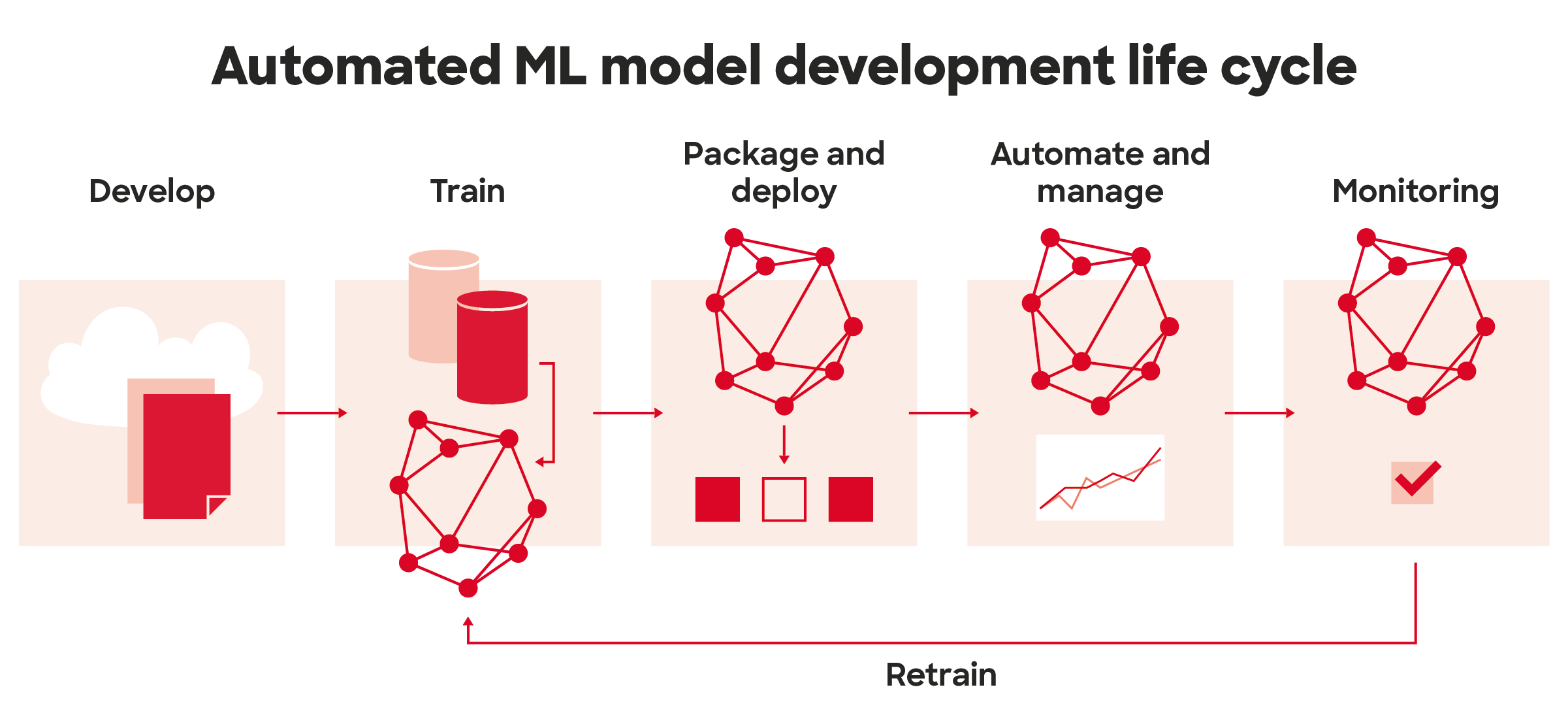
MLOps can be divided into multiple practices: automated infrastructure building, versioning important parts of data science experiments and models, deployments (packaging, continuous integration and continuous delivery), security and monitoring.

Versioning

In software development projects it is typical that source code, its configurations and also infrastructure code are versioned. Tracking and controlling changes to the code enables roll-backs to previous versions in case of failures and helps developers to understand the evolution of the solution. In data science projects source code and infrastructure are important to version as well, but in addition to them, there are other parts that need to be versioned, too.

Typically a data scientist runs training jobs multiple times with different setups. For example hyperparameters and used features may vary between different runs and they affect the accuracy of the model. If the information about training data, hyperparameters, model itself and model accuracy with different combinations are not saved anywhere it might be hard to compare the models and choose the best one to deploy to production.

Templates and shared libraries

Data scientists might lack knowledge on infrastructure development or networking, but if there is a ready template and framework, they only need to adapt the steps of a process. Templating and using shared libraries frees time from data scientists so they can focus on their core expertise.

Existing templates and shared libraries that abstract underlying infrastructure, platforms and databases, will speed up building new machine learning models but will also help in on-boarding any new data scientists.

Project templates can automate the creation of infrastructure that is needed for running the preprocessing or training code. When for example building infrastructure is automated with Infrastructure as a code, it is easier to build different environments and be sure they’re similar. This usually means also infrastructure security practices are automated and they don’t vary from project to project.

Templates can also have scripts for packaging and deploying code. When the libraries used are mostly the same in different projects, those scripts very rarely need to be changed and data scientists don’t have to write them separately for every project.

Shared libraries mean less duplicate code and smaller chance of bugs in repeating tasks. They can also hide details about the database and platform from data scientists, when they can use ready made functions for, for instance, reading from and writing to database or saving the model. Versioning can be written into shared libraries and functions as well, which means it’s not up to the data scientist to remember which things need to be versioned.

Deployment pipeline

When deploying either a more traditional software solution or ML solution, the steps in the process are highly repetitive, but also error-prone. An automated deployment pipeline in CI/CD service can take care of packaging the code, running automated tests and deployment of the package to a selected environment. This will not only reduce the risk of errors in deployment but also free time from the deployment tasks to actual development work.

Tests are needed in deployment of machine learning models as in any software, including typical unit and integration tests of the system. In addition to those, you need to validate data and the model, and evaluate the quality of the trained model. Adding the necessary validation creates a bit more complexity and requires automation of steps that are manually done before deployment by data scientists to train and validate new models. You might need to deploy a multi-step pipeline to automatically retrain and deploy models, depending on your solution.

Monitoring

After the model is deployed to production some people might think it remains functional and decays like any traditional software system. In fact, machine learning models can decay in more ways than traditional software systems. In addition to monitoring the performance of the system, the performance of models themselves needs to be monitored as well. Because machine learning models make assumptions of real-world based on the data used for training the models, when the surrounding world changes, accuracy of the model may decrease. This is especially true for the models that try to model human behavior. Decreasing model accuracy means that the model needs to be retrained to reflect the surrounding world better and with monitoring the retraining is not done too seldom or often. By tracking summary statistics of your data and monitoring the performance of your model, you can send notifications or roll back when values deviate from the expectations made in the time of last model training.

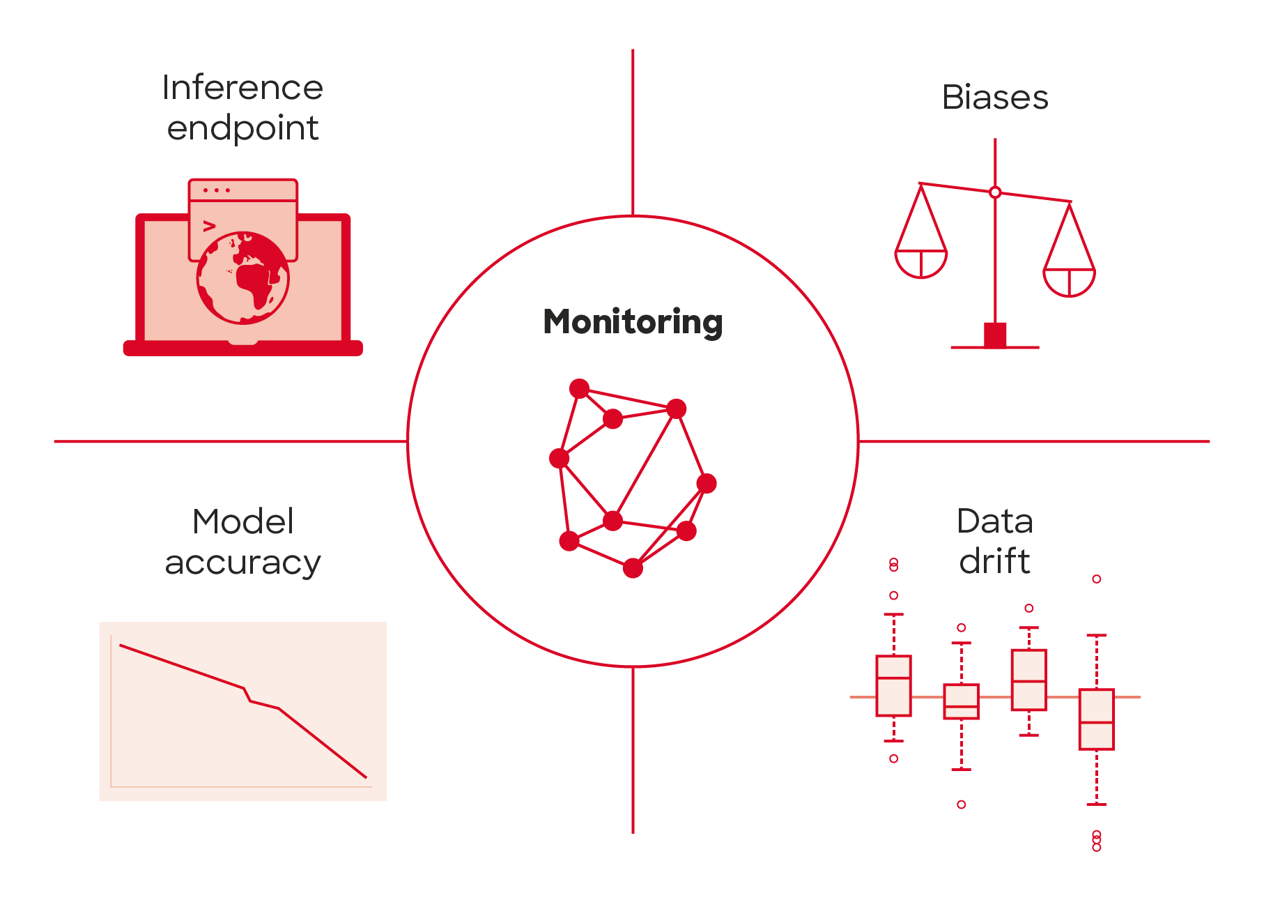
Applying MLOps

Bringing MLOps thinking to the machine learning model development enables you to actually get your models to production if you are not there yet, makes your deployment cycles faster and more reliable, reduces manual effort and errors, and frees time from your data scientists from tasks that are not their core competences to actual model development work. Cloud providers (such as AWS, Azure or GCP) are especially good places to start implementing MLOps in small steps, with ready made software components you can use. Moreover, all the CPU / GPU that is needed for model training with pay as you go model.

If the maturity of your AI journey is still in early phase (PoCs don’t need heavy processes like this), robust development framework and pipeline infra might not be the highest priority. However, any effort invested in automating the development process from the early phase will pay back later and reduce the machine learning technical debt in the long run. Start small and change the way you develop ML models towards MLOps by at least moving the development work on top of version control, and automating the steps for retraining and deployment.

DevOps was born as a reaction to systematic organization needed around rapidly expanding software development, and now the same problems are faced in the field of machine learning. Take the needed steps towards MLOps, like done successfully with DevOps before.

Lessons learned from combining SQS and Lambda in a data project

In June 2018, AWS Lambda added Amazon Simple Queue Service (SQS) to supported event sources, removing a lot of heavy lifting of running a polling service or creating extra SQS to SNS mappings. In a recent project we utilized this functionality and configured our data pipelines to use AWS Lambda functions for processing the incoming data items and SQS queues for buffering them. The built-in functionality of SQS and Lambda provided us serverless, scalable and fault-tolerant basis, but while running the solution we also learned some important lessons. In this blog post I will discuss the issue of valid messages ending up in dead-letter queues (DLQ) and correctly configuring your DLQ to catch only erroneous messages from your source SQS queue.

January 8, 2020

Miia Niemelä

What are Amazon SQS and Lambda?

In brief, Amazon SQS is a lightweight, fully managed message queueing service, that enables decoupling and scaling microservices, distributed systems and serverless applications. With SQS, it is easy to send, store, and receive messages between software components, without losing messages.

AWS Lambda is a fully managed, automatically scaling service that lets you run code in multiple different languages in a serverless manner, without having to provision any servers. You can configure a Lambda function to execute on response to various events or orchestrate the invocations. Your code runs in parallel and processes each invocation individually, scaling with the size of the workload.

When you configure an SQS queue as an event source for your Lambda, Lambda functions are automatically triggered when messages arrive to the SQS queue. The Lambda service automatically scales up and down based on the number of inflight messages in the queue. The polling, reading and removing of messages from the queue will be thus automatically handled by the built-in functionality. Successfully processed messages will be removed and the failed ones will be returned to the queue or forwarded to the DLQ, without needing to explicitly configure these steps inside your Lambda function code.

Problems with valid messages ending up in DLQ

In the recent project we needed to process data that would be coming in daily as well as in larger batches with historical data loadings through the same data processing pipeline. In order to handle changing data loads, SQS decouples the source system from processing and balances the load for both use cases. We used SQS for queueing metadata of new data files and Lambda function for processing the messages and passing on metadata to next steps in the pipeline. When testing our solution with pushing thousands of messages rapidly to the queue, we observed many of the messages ending up in a dead-letter queue, even though they were not erroneous.

From the CloudWatch metrics, we found no execution errors during the given period, but instead there was a peak in the Lambda throttling metric. We had configured a DLQ to catch erroneous messages, but ended up having completely valid and unprocessed messages in the DLQ. How does this happen? To understand this, let’s dive deeper into how Lambda functions are triggered and scaled when they have SQS configured as the event source.

Lambda scales automatically with the number of messages arriving to SQS – up to a limit

Let’s first introduce briefly the parameters of SQS and Lambda that are relevant to this problem.

SQS

ReceiveMessageWaitTimeSeconds: Time that the poller waits for new messages before returning a response. Your messages might be arriving to the SQS queue unevenly, sometimes in bursts and sometimes there might be no messages arriving at all. The default value is 0, which equals constant polling of messages. If the queue is empty and your solution allows some lag time, it might be beneficial not to poll the queue all the time and return empty responses. Instead of polling for messages constantly, you can specify a wait time between 1 and 20 seconds.

VisibilityTimeout: The length of time during which a message will be invisible to consumers after the message is read from the queue. When a poller reads a message from the SQS queue, that message still stays in the queue but becomes invisible for the period of VisibilityTimeout. During this time the read message will be unavailable for any other poller trying to read the same message and gives the initial component time to process and delete the message from the queue.

maxReceiveCount: Defines the number of times a message can be delivered back to being visible in the source queue before moving it to the DLQ. If the processing of the message is successful, the consumer will delete it from the queue. When ever an error occurs in processing of a message and it cannot be deleted from the queue, the message will become visible again in the queue with an increased ReceiveCount. When the ReceiveCount for a message exceeds the maxReceiveCount for a queue, message is moved to a dead-letter queue.

Lambda

Reserved concurrency limit: The number of executions of the Lambda function that can run simultaneously. There is an account specific limit how many executions of Lambda functions can run simultaneously (by default 1,000) and it is shared between all your Lambda functions. By reserving part of it for one function, other functions running at the same time can’t prevent your function from scaling.

BatchSize: The maximum number of messages that Lambda retrieves from the SQS queue in a single batch. Batchsize is related to the Lambda event source mapping, which defines what triggers the Lambda functions. In this case they are triggered from SQS.

In the Figure 1 below, it is illustrated how Lambda actually scales when messages arrive in bursts to the SQS queue. Lambda uses long polling to poll messages in the queue, which means that it does not poll the queue all the time but instead on an interval between 1 to 20 seconds, depending on what you have configured to be your queue’s ReceiveMessageWaitTimeSeconds. Lambda service’s internal poller reads messages as batches from the queue and invokes the Lambda function synchronously with an event that contains a batch of messages. The number of messages in a batch is defined by the BatchSize that is configured in the Lambda event source mapping.

When messages start arriving to the queue, Lambda reads first up to 5 batches and invokes a function for each. If there are messages still available, the number of processes reading the batches are increased by up to 60 more instances per minute (Figure 2), until it reaches the 1) reserved concurrency limit configured for the Lambda function in question or 2) the account’s limit of total concurrent Lambda executions (by default 1,000), whichever is lower (N in the figure).

By setting up a reserved concurrency limit for your Lambda, you guarantee that it will get part of the account’s Lambda resources at any time, but at the same time you also limit your function from scaling over that limit, even though there would be Lambda resources available for your account to use. When that limit is reached and there are still messages available in the queue, one might assume that those messages will stay visible in the queue, waiting until there’s free Lambda capacity available to handle those messages. Instead, the internal poller still tries to invoke new Lambda functions for all the new messages and therefore causes throttling of the Lambda invokes (figure 2). Why are some messages ending up in DLQ then?

Let’s look at how the workflow goes for an individual message batch if it succeeds or fails (figure 3). First, the Lambda internal poller reads a message batch from the queue and those messages stay in the queue but become invisible for the length of the configured VisibilityTimeout. Then it invokes a function synchronously, meaning that it will wait for a response that indicates a successful processing or an error, that can be caused by e.g. function code error, function timeout or throttling. In the case of a successful processing, the message batch is deleted from the queue. In the case of failure, however, the message becomes visible again.

The SQS queue is not aware of what happens beyond the event source mapping, if the invocations are failed or throttled. It keeps the messages in the queue invisible, until they get either deleted or turned back to visible after the length of VisibilityTimeout has passed. Effectually this means that throttled messages are treated as any other failed messages, so their ReceiveCount is increased every time they are made visible in the queue. If there is a huge burst of messages coming in, some of the messages might get throttled, retried, throttled again, and retried again, until they reach the limit of maxReceiveCount and then moved to the DLQ.

The automatic scaling and concurrency achieved with SQS and Lambda sounds promising, but unfortunately like all AWS services, this combination has its limits as well. Throttling of valid messages can be avoided with the following considerations:

Be careful when configuring a reserved concurrency to your Lambda function: the smaller the concurrency, the greater the chance that the messages get throttled. AWS suggests the reserved concurrency for a Lambda function to be 5 or greater.

Set the maxReceiveCount big enough in your SQS queue’s properties, so that the throttled messages will eventually get processed after the burst of messages. AWS suggest you set it to 5 or greater.

By increasing message VisibilityTimeout of the source queue, you can give more time for your Lambda to retry the messages in the case of message bursts. AWS suggests this to be set to at least 6 times the timeout you configure to your Lambda function.

Of course, tuning these parameters is an act of balancing with what best suits the purpose of your application.

Configuring DLQ to your SQS and Lambda combination

If you don’t configure a DLQ, you will lose all the erroneous (or valid and throttled) messages. If you are familiar with the topic this seems obvious, but it’s worth stating since it is quite important. What is confusing now in this combo, is that you can configure a dead-letter queue to both SQS and Lambda. The AWS documentation states:

“Make sure that you configure the dead-letter queue on the source queue, not on the Lambda function. The dead-letter queue that you configure on a function is used for the function’s asynchronous invocation queue, not for event source queues.“

To understand this one needs to dive into the difference between synchronous and asynchronous invocation of Lambda functions.

When you invoke a function synchronously Lambda runs the function and waits for a response from it. The function code returns the response, and Lambda returns you this response with some additional data, including e.g. the function version. In the case of asynchronous invocation, however, Lambda sends the invocation event to an internal queue. If the event is successfully sent to the internal queue, Lambda returns success response without waiting for any response from the function execution, unlike in synchronous invocation. Lambda manages the internal queue and attempts to retry failed events automatically with its own logic. If the execution of the function is failing after retries as well, the event is sent to the DLQ configured to the Lambda function. With event source mapping to SQS, Lambda is invoked synchronously, therefore there are no retries like in asynchronous invocation and the DLQ on Lambda is useless.

Recently, AWS launched Lambda Destinations, that makes it possible to route asynchronous function results to a destination resource that can be either SQS, SNS, another Lambda function or EventBridge. With DLQs you can handle asynchronous failure situations and catch the failing events, but with Destinations you can actually get more detailed information on function execution in both success and failure, such as code exception stack traces. Although, Destinations and DLQs can be used together and at the same time, AWS suggests Destinations should be considered a more preferred solution.

Conclusions

The described problems are all stated and deductible from the AWS documentation, but still not completely obvious. With carefully tuning the parameters of our SQS queue, mainly by increasing the maxReceiveCount and VisibilityTimeOut, we were able to overcome the problems with Lambda functions throttling. With configuring the DLQ to the source SQS queue instead of configuring it to Lambda, we were able to catch erroneous or throttled messages. Although adding a DLQ to your source SQS does not solve anything by itself, but you also need to handle the failing messages in some way. We configured a Lambda function also to the DLQ to write the erroneous messages to DynamoDB. This way we have a log of the unhandled messages in DynamoDB and the messages can be resubmitted or investigated further from there.

Of course, there are always several kinds of architectural options to solve these kind of problems in AWS environment. Amazon Kinesis, for example, is a real-time stream processing service, but designed to ingest large volumes of continuous streaming data. Our data, however, comes in uneven bursts, and SQS acts better for that scenario as a message broker and decoupling mechanism. One just needs to be careful with setting up the parameters correctly, as well as be sure that the actions intended for the Lambda function will execute within Lambda limits (including 15 minutes timeout and 3,008 MB maximum memory allocation). The built-in logic with Lambda and SQS enabled the minimal infrastructure to manage and monitor as well as high concurrency capabilities within the given limits.

AWS launches major new features for Amazon SageMaker to simplify development of machine learning models

Machine learning continues to grow on AWS and they are putting serious effort on paving the way for customers’ machine learning development journey on AWS cloud. The Andy Jassy keynote in AWS Re:Invent was a fiesta for data scientists with the newly launched Amazon SageMaker features, including Experiments, Debugger, Model Monitor, AutoPilot and Studio.

December 9, 2019

Miia Niemelä

Anniina Sallinen

AWS really aims to make the whole development life cycle of machine learning models as simple as possible for data scientists. With the newly launched features, they are addressing common, effort demanding problems: monitoring your data validity from your model’s perspective and monitoring your model performance (Model Monitor), experimenting multiple machine learning approaches in parallel for your problem (Experiments), enable cost efficiency of heavy model training with automatic rules (Debugger) and following these processes in a visual interface (Studio). These processes can even be orchestrated for you with AutoPilot, that unlike many services is not a black box machine learning solution but provides all the generated code for you. Announced features also included a SSO integrated login to SageMaker Studio and SageMaker Notebooks, a possibility to share notebooks with one click to other data scientists including the needed runtime dependencies and libraries (preview).

Compare and try out different models with SageMaker Experiments

Building a model is an iterative process of trials with different hyperparameters and how they affect the performance of the model. SageMaker Experiments aim to simplify this process. With Experiments, one can create trial runs with different parameters and compare those. It provides information about the hyperparameters and performance for each trial run, regardless of whether a data scientist has run training multiple times, has used automated hyperparameter tuning or has used AutoPilot. It is especially helpful in the case of automating some steps or the whole process, because the amount of training jobs run is typically much higher than with traditional approach.

Experiments makes it easy to compare trials, see what kind of hyperparameters was used and monitor the performance of the models, without having to set up the versioning manually. It makes it easy to choose and deploy the best model to production, but you can also always come back and look at the artifacts of your model when facing problems in production. It also provides more transparency for example to automated hyperparameter tuning and also for new SageMaker AutoPilot. Additionally, SageMaker Experiments has Experiments SDK so it is possible call the API with Python to get the best model programmatically and deploy endpoint for it.

Track issues in model training with SageMaker Debugger

During the training process of your model, many issues may occur that might prevent your model from correctly finishing or learning patterns. You might have, for example, initialized parameters inappropriately or used un efficient hyperparameters during the training process. SageMaker Debugger aims to help tracking issues related to your model training (unlike the name indicates, SageMaker Debugger does not debug your code semantics).

When you enable debugger in your training job, it starts to save the internal model state into S3 bucket during the training process. A state consists of for example weights for neural network, accuracies and losses, output of each layer and optimization parameters. These debug outputs will be analyzed against a collection of rules while the training job is executed. When you enable Debugger while running your training job in SageMaker, will start two jobs: a training job, and a debug processing job (powered by Amazon SageMaker Processing Jobs), which will run in parallel and analyze state data to check if the rule conditions are met. If you have, for example, an expensive and time consuming training job, you can set up a debugger rule and configure a CloudWatch alarm to it that kills the job once your rules trigger, e.g. loss has converged enough.

For now, the debugging framework of saving internal model states supports only TensorFlow, Keras, Apache MXNet, PyTorch and XGBoost. You can also configure your own rules that analyse model states during the training, or some preconfigured ones such as loss not changing or exploding/vanishing gradients. You can use the debug feature visually through the SageMaker Studio or alternatively through SDK and configure everything to it yourself.

Keep your model up-to-date with SageMaker Model Monitor

Drifts in data might have big impact on your model performance in production, if your training data and validation data start to have different statistical properties. Detecting those drifts requires efforts, like setting up jobs that calculate statistical properties of your data and also updating those, so that your model does not get outdated. SageMaker Model Monitor aims to solve this problem by tracking the statistics of incoming data and aims to ensure that machine learning models age well.

The Model Monitor forms a baseline from the training data used for creating a model. Baseline information includes statistics of the data and basic information like name and datatype of features in data. Baseline is formed automatically, but automatically generated baseline can be changed if needed. Model Monitor then continuously collects input data from deployed endpoint and puts it into a S3 bucket. Data scientists can then create own rules or use ready-made validations for the data and schedule validation jobs. They can also configure alarms if there are deviations from the baseline. These alarms and validations can indicate that the model deployed is actually outdated and should be re-trained.

SageMaker Model Monitor makes monitoring the model quality very easy but at the same time data scientists have the control and they can customize the rules, scheduling and alarms. The monitoring is attached to an endpoint deployed with SageMaker, so if inference is implemented in some other way, Model Monitor cannot be used. SageMaker endpoints are always on, so they can be expensive solution for cases when predictions are not needed continuously.

Start from scratch with SageMaker AutoPilot

SageMaker AutoPilot is an autoML solution for SageMaker. SageMaker has had automatic hyperparameter tuning already earlier, but in addition to that, AutoPilot takes care of preprocessing data and selecting appropriate algorithm for the problem. This saves a lot of time of preprocessing the data and enables building models even if you’re not sure which algorithm to use. AutoPilot supports linear learner, factorization machines, KNN and XGBboost at first, but other algorithms will be added later.

Running an AutoPilot job is as easy as just specifying a csv-file and response variable present in the file. AWS considers that models trained by SageMaker AutoPilot are white box models instead of black box, because it provides generated source code for training the model and with Experiments it is easy to view the trials AutoPilot has run.

SageMaker AutoPilot automates machine learning model development completely. It is yet to be seen if it improves the models, but it is a good sign that it provides information about the process. Unfortunately, the description of the process can only be viewed in SageMaker Studio (only available in Ohio at the moment). Supported algorithms are currently quite limited as well, so the AutoPilot might not provide the best performance possible for some problems. In practice running AutoPilot jobs takes a long time, so the costs of using AutoPilot might be quite high. That time is of course saved from data scientist’s working time. One possibility is, for example, when approaching a completely new data set and problem, one might start by launching AutoPilot and get a few models and all the codes as template. That could serve as a kick start to iterating your problem by starting from tuning the generated code and continuing development from there, saving time from initial setup.

SageMaker Studio – IDE for data science development

The launched SageMaker Studio (available in Ohio) is a fully integrated development environment (IDE) for ML, built on top of Jupyter lab. It pulls together the ML workflow steps in a visual interface, with it’s goal being to simplify the iterative nature of ML development. In Studio one can move between steps, compare results and adjust inputs and parameters. It also simplifies the comparison of models and runs side by side in one visual interface.

Studio seems to nicely tie the newly launched features (Experiments, Debugger, Model Monitor and Autopilot) into a single web page user interface. While these new features are all usable through SDKs, using them through the visual interface will be more insightful for a data scientist.

Conclusion

These new features enable more organized development of machine learning models, moving from notebooks to controlled monitoring and deployment and transparent workflows. Of course several actions enabled by these features could be implemented elsewhere (e.g. training job debugging, or data quality control with some scheduled smoke tests), but it requires again more coding and setting up infrastructure. The whole public cloud journey of AWS has been aiming to simplify development and take load away by providing reusable components and libraries, and these launches go well with that agenda.